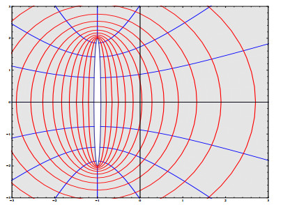
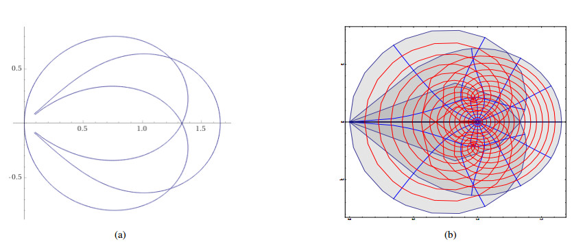
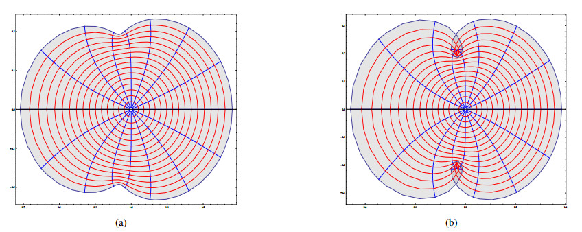
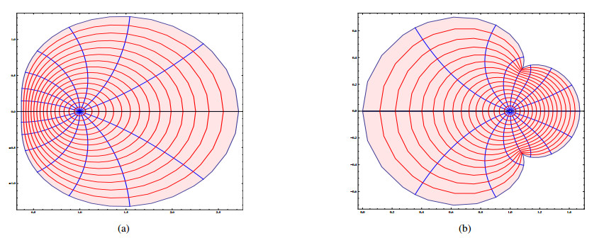
The purpose of this present paper is to investigate some mapping properties of functions which map the unit disc onto a overlapped leaf-like curve, having real part greater than zero. Also we define a class of $ \lambda $-pseudo starlike functions related to a leaf-like curve. Integral representation, inequalities for the initial Taylor-Maclaurin coefficients and Fekete-Szegö problem for subclasses of analytic functions related to various conic regions are obtained as our main results.
Citation: N. E. Cho, G. Murugusundaramoorthy, K. R. Karthikeyan, S. Sivasubramanian. Properties of $ \lambda $-pseudo-starlike functions with respect to a boundary point[J]. AIMS Mathematics, 2022, 7(5): 8701-8714. doi: 10.3934/math.2022486
The purpose of this present paper is to investigate some mapping properties of functions which map the unit disc onto a overlapped leaf-like curve, having real part greater than zero. Also we define a class of $ \lambda $-pseudo starlike functions related to a leaf-like curve. Integral representation, inequalities for the initial Taylor-Maclaurin coefficients and Fekete-Szegö problem for subclasses of analytic functions related to various conic regions are obtained as our main results.

| [1] | Z. Nehari, Conformal mapping, McGraw-Hill Book Co., Inc., New York, Toronto, London, 1952. |
| [2] | A. W. Goodman, Univalent functions Vol. II, Mariner Publishing Co., Inc., Tampa, FL, 1983. |
| [3] |
M. S. Robertson, Univalent functions starlike with respect to a boundary point, J. Math. Anal. Appl., 81 (1981), 327–345. https://doi.org/10.1016/0022-247X(81)90067-6 doi: 10.1016/0022-247X(81)90067-6

|
| [4] | M. H. Annaby, Z. S. Mansour, $q$-fractional calculus and equations, Lecture Notes in Mathematics, Springer, Heidelberg, 2012. |
| [5] | A. Aral, V. Gupta, R. P. Agarwal, Applications of $q$-calculus in operator theory, Springer, New York, 2013. |
| [6] | F. H. Jackson, On $q$-definite integrals, Quart. J. Pure Appl. Math., 41 (1910), 193–203. |
| [7] | H. M. Srivastava, Univalent functions, fractional calculus, and associated generalized hypergeometric functions, John Wiley and Sons, New York, 1989. |
| [8] |
H. M. Srivastava, Operators of basic (or $q$-) calculus and fractional $q$-calculus and their applications in geometric function theory of complex analysis, Iran. J. Sci. Technol. A, 44 (2020), 327–344. https://doi.org/10.1007/s40995-019-00815-0 doi: 10.1007/s40995-019-00815-0
|
| [9] |
S. M. Aydoğan, F. M. Sakar, Radius of starlikeness of $p$-valent $\lambda$-fractional operator, Appl. Math. Comput., 357 (2019), 374–378. https://doi.org/10.1016/j.amc.2018.11.067 doi: 10.1016/j.amc.2018.11.067
|
| [10] |
K. R. Karthikeyan, M. Ibrahim, K. Srinivasan, Fractional class of analytic functions defined using $q$-differential operator, Aust. J. Math. Anal. Appl., 15 (2018). https://doi.org/10.1007/s00009-018-1200-2 doi: 10.1007/s00009-018-1200-2
|
| [11] |
K. R. Karthikeyan, G. Murugusundaramoorthy, N. E. Cho, Some inequalities on Bazilevič class of functions involving quasi-subordination, AIMS Math., 6 (2021), 7111–7124. https://doi.org/10.3934/math.2021417 doi: 10.3934/math.2021417
|
| [12] |
K. R. Karthikeyan, G. Murugusundaramoorthy, T. Bulboacă, Properties of $\lambda$-pseudo-starlike functions of complex order defined by subordination, Axioms, 10 (2021), 86. https://doi.org/10.3390/axioms10020086 doi: 10.3390/axioms10020086
|
| [13] |
K. A. Reddy, K. R. Karthikeyan, G. Murugusundaramoorthy, Inequalities for the Taylor coefficients of spiralike functions involving $q$-differential operator, Eur. J. Pure Appl. Math., 12 (2019), 846–856. https://doi.org/10.29020/nybg.ejpam.v12i3.3429 doi: 10.29020/nybg.ejpam.v12i3.3429
|
| [14] | F. M. Sakar, M. Naeem, S. Khan, S. Hussain, Hankel determinant for class of analytic functions involving $q$-derivative operator, J. Adv. Math. Stud., 14 (2021), 265–278. |
| [15] | F. M. Sakar, A. Canbulat, Quasi-subordinations for a subfamily of bi-univalent functions associated with $k$-analogue of bessel function, J. Math. Anal., 12 (2021), 1–12. |
| [16] |
H. M. Srivastava, B. Khan, N. Khan, Q. Z. Ahmad, M. Tahir, A generalized conic domain and its applications to certain subclasses of analytic functions, Rocky Mountain J. Math., 49 (2019), 2325–2346. https://doi.org/10.1216/RMJ-2019-49-7-2325 doi: 10.1216/RMJ-2019-49-7-2325
|
| [17] |
H. M. Srivastava, Q. Z. Ahmad, N. Khan, N. Khan, B. Khan, Hankel and Toeplitz determinants for a subclass of q-starlike functions associated with a general conic domain, Mathematics, 7 (2019), 181. https://doi.org/10.3390/math7020181 doi: 10.3390/math7020181
|
| [18] |
H. M. Srivastava, B. Khan, N. Khan, Q. Z. Ahmad, Coefficient inequalities for $q$-starlike functions associated with the Janowski functions, Hokkaido Math. J., 48 (2019), 407–425. https://doi.org/10.14492/hokmj/1562810517 doi: 10.14492/hokmj/1562810517
|
| [19] | W. C. Ma, D. Minda, A unified treatment of some special classes of univalent functions, Proceedings of the Conference on Complex Analysis, Conf. Proc. Lecture Notes Anal., I, Int. Press, Cambridge, MA, 1992. |
| [20] |
A. Lecko, G. Murugusundaramoorthy, S. Sivasubramanian, On a class of analytic functions related to Robertson's formula and subordination, Bol. Soc. Mat. Mex., 8 (2021). https://doi.org/10.1007/s40590-021-00331-5 doi: 10.1007/s40590-021-00331-5
|
| [21] |
A. Lecko, G. Murugusundaramoorthy, S. Sivasubramanian, On a subclass of analytic functions that are starlike with respect to a boundary point involving exponential function, J. Funct. Space., 2022 (2022). https://doi.org/10.1155/2022/4812501 doi: 10.1155/2022/4812501
|
| [22] |
K. O. Babalola, On $\lambda$-pseudo-starlike functions, J. Class. Anal., 3 (2013), 137–147. https://doi.org/10.7153/jca-03-12 doi: 10.7153/jca-03-12
|
| [23] | C. Pommerenke, Univalent functions, Vandenhoeck & Ruprecht, Göttingen, 1975. |
| [24] |
S. Agrawal, S. K. Sahoo, A generalization of starlike functions of order alpha, Hokkaido Math. J., 46 (2017), 15–27. https://doi.org/10.14492/hokmj/1498788094 doi: 10.14492/hokmj/1498788094
|
Figures(4)

N. E. Cho, G. Murugusundaramoorthy, K. R. Karthikeyan, S. Sivasubramanian. Properties of $ \lambda $-pseudo-starlike functions with respect to a boundary point[J]. AIMS Mathematics, 2022, 7(5): 8701-8714. doi: 10.3934/math.2022486


 DownLoad: