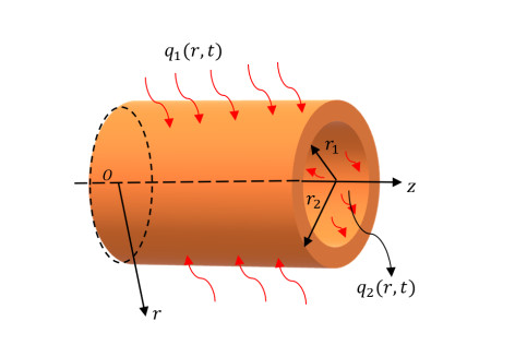
In this paper, a new fractional model of non-Fourier heat conduction is presented that includes phase delays and two fractional orders. To derive the proposed model, the fractional integral Atangana-Baleanu (AB) operator with non-singular and non-local kernels was used. The proposed model has been applied to solve a one-dimensional thermoelasticity problem that includes an annular cylinder of a flexible material whose inner and outer surfaces are subjected to a variable heat flux that depends on time and temperature and is free from traction. The Laplace transform approach was applied to find the general solution to the problem and to obtain the expressions for the different physical fields. To estimate the effects of the fractional-order parameters and instantaneous time on the responses of all thermophysical field variables, comparisons are presented in figures and tables.
Citation: Ahmed Abouelregal, Meshari Alesemi, Husam Alfadil. Thermoelastic reactions in a long and thin flexible viscoelastic cylinder due to non-uniform heat flow under the non-Fourier model with fractional derivative of two different orders[J]. AIMS Mathematics, 2022, 7(5): 8510-8533. doi: 10.3934/math.2022474
In this paper, a new fractional model of non-Fourier heat conduction is presented that includes phase delays and two fractional orders. To derive the proposed model, the fractional integral Atangana-Baleanu (AB) operator with non-singular and non-local kernels was used. The proposed model has been applied to solve a one-dimensional thermoelasticity problem that includes an annular cylinder of a flexible material whose inner and outer surfaces are subjected to a variable heat flux that depends on time and temperature and is free from traction. The Laplace transform approach was applied to find the general solution to the problem and to obtain the expressions for the different physical fields. To estimate the effects of the fractional-order parameters and instantaneous time on the responses of all thermophysical field variables, comparisons are presented in figures and tables.

| [1] | Y. Povstenko, Fractional thermoelasticity, New York: Springer 2015. |
| [2] |
Y. Povstenko, Theories of thermal stresses based on space-time-fractional telegraph equations, Comput. Math. Appl., 64 (2012), 3321-3328. https://doi.org/10.1016/j.camwa.2012.01.066 doi: 10.1016/j.camwa.2012.01.066

|
| [3] |
H. W. Lord, Y. Shulman, A generalized dynamical theory of thermoelasticity, J. Mech. Phys. Solids, 15 (1967), 299-309. https://doi.org/10.1016/0022-5096(67)90024-5 doi: 10.1016/0022-5096(67)90024-5
|
| [4] | A. E. Green, K. A. Lindsay, Thermoelasticity, J. Elasticity, 2 (1972), 1-7. https://doi.org/10.1007/BF00045689 |
| [5] |
A. E. Green, P. M. Naghdi, A re-examination of the basic postulates of thermomechanics, Proc. R. Soc. A, Math. Phys. Eng. Sci., 432 (1991), 171-194. https://doi.org/10.1098/rspa.1991.0012 doi: 10.1098/rspa.1991.0012
|
| [6] |
A. E. Green, P. M. Naghdi, On undamped heat waves in an elastic solid, J. Therm. Stresses, 15 (1992), 253-264. https://doi.org/10.1080/01495739208946136 doi: 10.1080/01495739208946136
|
| [7] |
A. E. Green, P. M. Naghdi, Thermoelasticity without energy dissipation, J. Elasticity, 31 (1993), 189-208. https://doi.org/10.1007/BF00044969 doi: 10.1007/BF00044969
|
| [8] |
D. Y. Tzou, A unified field approach for heat conduction from macro- to micro-scales, J. Heat Transfer, 117 (1995), 8-16. https://doi.org/10.1115/1.2822329 doi: 10.1115/1.2822329
|
| [9] |
D. S. Chandrasekharaiah, Hyperbolic thermoelasticity: A review of recent literature, Appl. Mech. Rev., 51 (1998), 705-729. https://doi.org/10.1115/1.3098984 doi: 10.1115/1.3098984
|
| [10] |
R. B. Hetnarski, J. Ignaczak, Generalized thermoelasticity, J. Therm. Stresses, 22 (1999), 451-476. https://doi.org/10.1080/014957399280832 doi: 10.1080/014957399280832
|
| [11] |
A. E. Abouelregal, Two-temperature thermoelastic model without energy dissipation including higher order time-derivatives and two phase-lags, Mater. Res. Express, 6 (2019), 116535. https://doi.org/10.1088/2053-1591/ab447f doi: 10.1088/2053-1591/ab447f
|
| [12] | A. E. Abouelregal, A novel generalized thermoelasticity with higher-order time-derivatives and three-phase lags, Multidiscip. Model. Ma., 16 (2020), 689-711. |
| [13] |
A. E. Abouelregal, Three-phase-lag thermoelastic heat conduction model with higher-order time-fractional derivatives, Indian J. Phys., 94 (2020), 1949-1963. https://doi.org/10.1007/s12648-019-01635-z doi: 10.1007/s12648-019-01635-z
|
| [14] |
H. Zhou, P. Li, Nonlocal dual-phase-lagging thermoelastic damping in rectangular and circular micro/nanoplate resonators, Appl. Math. Model., 95 (2021), 667-687. https://doi.org/10.1016/j.apm.2021.02.035 doi: 10.1016/j.apm.2021.02.035
|
| [15] |
H. Zhou, P. Li, Y. Fang, Single-phase-lag thermoelastic damping models for rectangular cross-sectional micro- and nano-ring resonators, Int. J. Mech. Sci., 163 (2019), 105132. https://doi.org/10.1016/j.ijmecsci.2019.105132 doi: 10.1016/j.ijmecsci.2019.105132
|
| [16] |
H. Zhou, P. Li, W. Zuo, Y. Fang, Dual-phase-lag thermoelastic damping models for micro/nanobeam resonators, Appl. Math. Model., 79 (2020), 31-51. https://doi.org/10.1016/j.apm.2019.11.027 doi: 10.1016/j.apm.2019.11.027
|
| [17] |
H. Zhou, P. Li, Dual-phase-lagging thermoelastic damping and frequency shift of micro/nano-ring resonators with rectangular cross-section, Thin-Wall. Struct., 159 (2021), 107309. https://doi.org/10.1016/j.tws.2020.107309 doi: 10.1016/j.tws.2020.107309
|
| [18] |
S. Deswal, K. K. Kalkal, R. Yadav, Response of fractional ordered micropolar thermoviscoelastic half-space with diffusion due to ramp type mechanical load, Appl. Math. Model., 49 (2017), 144-161. https://doi.org/10.1016/j.apm.2017.04.040 doi: 10.1016/j.apm.2017.04.040
|
| [19] |
S. Mesloub, F. Aldosari, On a two-dimensional fractional thermoelastic system with nonlocal constraints describing a fractional Kirchhoff plate, Adv. Differ. Equ., 2021 (2021), 24. https://doi.org/10.1186/s13662-020-03188-6 doi: 10.1186/s13662-020-03188-6
|
| [20] |
B. Ross, The development of fractional calculus 1695-1900, Hist. Math., 4 (1977) 75-89. https://doi.org/10.1016/0315-0860(77)90039-8 doi: 10.1016/0315-0860(77)90039-8
|
| [21] | K. S. Miller B. Ross, An introduction to the fractional calculus and fractional differential equations, John Wiley and Sons, New York, USA, 1993. |
| [22] | I. Podlubny, Fractional differential equations, New York, USA: Academic Press, 1999. |
| [23] |
Y. Z. Povstenko, Fractional radial heat conduction in an infinite medium with a cylindrical cavity and associated thermal stresses, Mech. Res. Commun., 37 (2010), 436-440. https://doi.org/10.1016/j.mechrescom.2010.04.006 doi: 10.1016/j.mechrescom.2010.04.006
|
| [24] |
M. Caputo, Linear models of dissipation whose Q is almost frequency independent-Ⅱ, Geophys. J. Int., 13 (1967), 529-539. https://doi.org/10.1111/j.1365-246X.1967.tb02303.x doi: 10.1111/j.1365-246X.1967.tb02303.x
|
| [25] |
H. H. Sherief, A. M. A. El-Sayed, A. M. Abd El-Latief, Fractional order theory of thermoelasticity, Int. J. Solids Struct., 47 (2010), 269-275. https://doi.org/10.1016/j.ijsolstr.2009.09.034 doi: 10.1016/j.ijsolstr.2009.09.034
|
| [26] |
M. A. Ezzat, Thermoelectric MHD non-Newtonian fluid with fractional derivative heat transfer, Phys. B, 405 (2010), 4188-4194. http://dx.doi.org/10.1016/j.physb.2010.07.009 doi: 10.1016/j.physb.2010.07.009
|
| [27] |
A. S. El-Karamany, M. A. Ezzat, Convolutional variational principle, reciprocal and uniqueness theorems in linear fractional two-temperature thermoelasticity, J. Therm. Stresses, 34 (2011), 264-284. https://doi.org/10.1080/01495739.2010.545741 doi: 10.1080/01495739.2010.545741
|
| [28] |
F. Hamza, M. Abdou, A. M. Abd El-Latief, Generalized fractional thermoelasticity associated with two relaxation times, J. Therm. Stresses, 37 (2014), 1080-1098. https://doi.org/10.1080/01495739.2014.936196 doi: 10.1080/01495739.2014.936196
|
| [29] |
H. M. Youssef, Theory of fractional order generalized thermoelasticity. J. Heat Transfer, 132 (2010), 61301. https://doi.org/10.1115/1.4000705 doi: 10.1115/1.4000705
|
| [30] |
Y. Z. Povstenko, Fractional heat conduction equation and associated thermal stress, J. Therm. Stresses, 28 (2004), 83-102. https://doi.org/10.1080/014957390523741 doi: 10.1080/014957390523741
|
| [31] |
A. E. Abouelregal, A modified law of heat conduction of thermoelasticity with fractional derivative and relaxation time, J. Mol. Eng. Mater., 8 (2020), 2050003. https://doi.org/10.1142/S2251237320500033 doi: 10.1142/S2251237320500033
|
| [32] |
K. Zakaria, M. A. Sirwah, A. E. Abouelregal, A. F. Rashid, Photo-thermoelastic model with time-fractional of higher order and phase lags for a semiconductor rotating materials, Silicon, 13 (2021), 573-585. https://doi.org/10.1007/s12633-020-00451-z doi: 10.1007/s12633-020-00451-z
|
| [33] |
A. E. Abouelregal, Modified fractional thermoelasticity model with multi-relaxation times of higher order: Application to spherical cavity exposed to a harmonic varying heat, Waves Random Complex, 31 (2021), 812-832. https://doi.org/10.1080/17455030.2019.1628320 doi: 10.1080/17455030.2019.1628320
|
| [34] |
A. E. Abouelregal, Fractional heat conduction equation for an infinitely generalized, thermoelastic, long solid cylinder, Int. J. Comput. Methods Eng. Sci. Mech., 17 (2016), 374-381. https://doi.org/10.1080/15502287.2012.698700 doi: 10.1080/15502287.2012.698700
|
| [35] | M. Caputo, M. Fabrizio, A new definition of fractional derivative without singular kernel, Prog. Fract. Differ. Appl., 1 (2015), 73-85. |
| [36] |
A. Atangana, D. Baleanu, Caputo-Fabrizio derivative applied to groundwater flow within a confined aquifer, J. Eng. Mech., 143 (2016), 1-16. https://doi.org/10.1061/(ASCE)EM.1943-7889.0001091 doi: 10.1061/(ASCE)EM.1943-7889.0001091
|
| [37] |
A. Atangana, D. Baleanu, New fractional derivatives with nonlocal and non-singular kernel: Theory and application to heat transfer model, Therm. Sci., 20 (2016), 763-769. https://doi.org/10.2298/TSCI160111018A doi: 10.2298/TSCI160111018A
|
| [38] |
A. Atangana, J. F. Gómez-Aguilar, Decolonisation of fractional calculus rules: Breaking commutativity and associativity to capture more natural phenomena, Eur. Phys. J. Plus, 133 (2018), 1-22. https://doi.org/10.1140/epjp/i2018-12021-3 doi: 10.1140/epjp/i2018-12021-3
|
| [39] |
A. Atangana, I. Koca, Chaos in a simple nonlinear system with Atangana-Baleanu derivatives with fractional order, Chaos Solit. Fract., 89 (2016), 447-454. https://doi.org/10.1016/j.chaos.2016.02.012 doi: 10.1016/j.chaos.2016.02.012
|
| [40] |
E. Uçar, S. Uçar, F. Evirgen, N. Özdemir, A fractional SAIDR model in the frame of Atangana-Baleanu derivative, Fractal Fract., 5 (2021), 32. https://doi.org/10.3390/fractalfract5020032 doi: 10.3390/fractalfract5020032
|
| [41] |
A. Fernandez, I. Husain, Modified Mittag-Leffler functions with applications in complex formulae for fractional calculus, Fractal Fract., 4 (2020), 45. https://doi.org/10.3390/fractalfract4030045 doi: 10.3390/fractalfract4030045
|
| [42] |
A. O. Akdemir, A. Karaoğlan, M. A. Ragusa, E. Set, Fractional integral inequalities via Atangana-Baleanu operators for convex and concave functions, J. Funct. Spaces, 2021 (2021), 1055434. https://doi.org/10.1155/2021/1055434 doi: 10.1155/2021/1055434
|
| [43] | K. A. Abro, M. H. Laghari, J. F. Gómez-Aguilar, Application of Atangana-Baleanu fractional derivative to carbon nanotubes based non-newtonian nanofluid: Applications in nanotechnology, J. Appl. Comput. Mech., 6 (2020), 1260-1269. |
| [44] | A. G. M. Selvam, S. B. Jacob, Stability of Atangana-Baleanu fractional order differential equation with numerical approximation, J. Phys.: Conf. Ser., 2070 (2021) 012086. |
| [45] |
M. A. Elhagary, Effect of Atangana-Baleanu fractional derivative on a two-dimensional thermoviscoelastic problem for solid sphere under axisymmetric distribution, Mech. Based Des. Struc., 2021. https://doi.org/10.1080/15397734.2021.1922288 doi: 10.1080/15397734.2021.1922288
|
| [46] | A. Kilbas, H. M. Srivastava, J. J. Trujillo, Theory and applications of fractional differential equations, Elsevier Science, Amsterdam, The Netherlands, 2006. |
| [47] |
A. Atangana, A. Akgul, K. M. Owolabi, Analysis of fractal fractional differential equations, Alex. Eng. J., 59 (2020), 1117-1134. https://doi.org/10.1016/j.aej.2020.01.005 doi: 10.1016/j.aej.2020.01.005
|
| [48] |
D. Y. Tzou, The generalized lagging response in small-scale and high-rate heating, Int. J. Heat Mass Tran., 38 (1995), 3231-3240. https://doi.org/10.1016/0017-9310(95)00052-B doi: 10.1016/0017-9310(95)00052-B
|
| [49] | D. Y. Tzou, Macro-to microscale heat transfer: The lagging behavior, Taylor & Francis, New York, 2014. |
| [50] | A. E. Abouelregal, H. Ahmad, A modified thermoelastic fractional heat conduction model with a single-lag and two different fractional-orders, J. Appl. Comput. Mech., 7 (2021), 1676-1686. |
| [51] |
M. A. Ezzat, A. S. El-Karamany, S. M. Ezzat, Two-temperature theory in magneto-thermoelasticity with fractional order dual-phase-lag heat transfer, Nuclear Eng. Design, 252 (2012), 267-277. http://dx.doi.org/10.1016/j.nucengdes.2012.06.012 doi: 10.1016/j.nucengdes.2012.06.012
|
| [52] |
H. H. Sherief, M. N. Anwar, A problem in generalized thermoelasticity for an infinitely long annular cylinder, Int. J. Eng. Sci., 26 (1988), 301-306. https://doi.org/10.1016/0020-7225(88)90079-1 doi: 10.1016/0020-7225(88)90079-1
|
| [53] |
G. Honig, U. Hirdes, A method for the numerical inversion of Laplace transforms, J. Comput. Appl. Math., 10 (1984), 113-132. https://doi.org/10.1016/0377-0427(84)90075-X doi: 10.1016/0377-0427(84)90075-X
|
| [54] |
A. E. Abouelregal, H. Ersoy, Ö. Civalek, Solution of Moore-Gibson-Thompson equation of an unbounded medium with a cylindrical hole, Mathematics, 9 (2021), 1536. https://doi.org/10.3390/math9131536 doi: 10.3390/math9131536
|


Figures(9) / Tables(4)

Ahmed Abouelregal, Meshari Alesemi, Husam Alfadil. Thermoelastic reactions in a long and thin flexible viscoelastic cylinder due to non-uniform heat flow under the non-Fourier model with fractional derivative of two different orders[J]. AIMS Mathematics, 2022, 7(5): 8510-8533. doi: 10.3934/math.2022474


 DownLoad: