A geometrical model of dishwasher spray arm for CornerWash

Hakan Ateş; Fatma Ateş; Hakan Ateş; Fatma Ateş

doi:10.3934/math.2022475

AIMS Mathematics

2022, Volume 7, Issue 5: 8534-8541. doi: 10.3934/math.2022475

Previous Article Next Article

Research article Special Issues

A geometrical model of dishwasher spray arm for CornerWash

Hakan Ateş ^{1
,
,},
Fatma Ateş ²

1.
Mechanical Engineer, Arçelik Company, Ankara, Turkey
2.
Department of Mathematics-Computer Sciences, Necmettin Erbakan University, Konya, Turkey

Received: 23 October 2021 Revised: 11 February 2022 Accepted: 16 February 2022 Published: 28 February 2022
MSC : 14H50, 53A17, 53B30, 53Z30

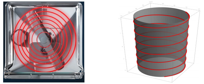
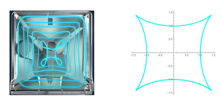
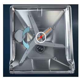
Many dishwasher manufacturers are in search of innovative solutions for issues such as washing performance, energy efficiency, water consumption and noise. The most critical place to make these improvements is in the spray arm design. With a good spray arm design, it can be reduced water consumption, energy consumption, and noise. In this study, we focus on a new spray arm design (studied by Arçelik) that increases efficiency. Also, we have obtained a geometrical interpretation of the new spray arm motion. We investigate the path followed by the new spray arm in $ 3- $dimensional Minkowski space and its projection on a plane. Finally, we present its three-dimensional and two-dimensional images.
- spherical timelike helix,
- dishwasher,
- cornerwash,
- hypocycloid,
- Minkowski $ 3- $space
Citation: Hakan Ateş, Fatma Ateş. A geometrical model of dishwasher spray arm for CornerWash[J]. AIMS Mathematics, 2022, 7(5): 8534-8541. doi: 10.3934/math.2022475

Related Papers:

Abstract

Many dishwasher manufacturers are in search of innovative solutions for issues such as washing performance, energy efficiency, water consumption and noise. The most critical place to make these improvements is in the spray arm design. With a good spray arm design, it can be reduced water consumption, energy consumption, and noise. In this study, we focus on a new spray arm design (studied by Arçelik) that increases efficiency. Also, we have obtained a geometrical interpretation of the new spray arm motion. We investigate the path followed by the new spray arm in $ 3- $dimensional Minkowski space and its projection on a plane. Finally, we present its three-dimensional and two-dimensional images.

References

[1]	P. Agarwal, M. A. Ramadan, A. A. M. Rageh, A. R. Hadhoud, A fractional-order mathematical model for analyzing the pandemic trend of COVID-19, Math. Meth. Appl. Sci., 2021, 1–18. https://doi.org/10.1002/mma.8057 doi: 10.1002/mma.8057
[2]	P. Agarwal, J. J. Nieto, M. Ruzhansky, D. F. M. Torres, Analysis of infectious disease problems (Covid-19) and their global impact, Singapore: Springer, 2021.
[3]	S. M. E. K. Chowdhury, J. T. Chowdhury, S. F. Ahmed, P. Agarwal, I. A. Badruddin, S. Kamangar, Mathematical modelling of COVID-19 disease dynamics: Interaction between immune system and SARS-CoV-2 within host, AIMS Math., 7 (2022), 2618–2633. https://doi.org/10.3934/math.2022147 doi: 10.3934/math.2022147
[4]	A. Rehman, R. Singh, P. Agarwal, Modeling, analysis and prediction of new variants of covid-19 and dengue co-infection on complex network, Chaos, Solitons Fract., 150 (2021), 111008. https://doi.org/10.1016/j.chaos.2021.111008 doi: 10.1016/j.chaos.2021.111008
[5]	Global Energy Transition Statistics, Enerdata Global Energy Statistical Yearbook, 2021. Available from: https://yearbook.enerdata.net/.
[6]	Total Energy Production, Enerdata Global Energy Statistical Yearbook, 2021. Available from: https://yearbook.enerdata.net/total-energy/world-energy-production.html.
[7]	C. P. Richter, Usage of dishwashers: Observation of consumer habits in the domestic environment, Int. J. Consum. Stud., 35 (2011), 180–186. https://doi.org/10.1111/j.1470-6431.2010.00973.x doi: 10.1111/j.1470-6431.2010.00973.x
[8]	Global Water Resources Under Increasing Pressure From Rapidly Growing Demands and Climate Change, According to New UN World Water Development Report, World Water Development Report (WWDR4), 2012. Available from: http://www.unesco.org.
[9]	K. J. Karlsson, Experimental study of how a motorized lower spray arm affects energy usage, wash result and sound level in a household dishwasher, Karlstad University, Master Thesis, 2021.
[10]	P. Tsouknidas, X. Zhang, Dishwasher improvement at ASKO–Developing a simplified test method to determine the influence of spray arm speed and pressure, Chalmers university of technology, Master Thesis, 2010.
[11]	R. Lopez, Differential geometry of curves and surfaces in Lorentz-Minkowski space, Int. Electron. J. Geom., 7 (2014), 44–107. https://doi.org/10.36890/iejg.594497 doi: 10.36890/iejg.594497
[12]	Ç. Camci, L. Kula, M. Altinok, On spacelike slant helices in $H_{0}^2$ and $S^2_{1}$, 2013, in press.
[13]	D. J. Struik, Lectures on classical differential geometry, New York: Dover Publications, 1988.

Reader Comments

Your name:*

Email:*
© 2022 the Author(s), licensee AIMS Press. This is an open access article distributed under the terms of the Creative Commons Attribution License (http://creativecommons.org/licenses/by/4.0)