New analysis of fuzzy fractional Langevin differential equations in Caputo's derivative sense

Muhammad Akram; Ghulam Muhammad; Tofigh Allahviranloo; Ghada Ali; Muhammad Akram; Ghulam Muhammad; Tofigh Allahviranloo; Ghada Ali

doi:10.3934/math.20221016

AIMS Mathematics

2022, Volume 7, Issue 10: 18467-18496. doi: 10.3934/math.20221016

Previous Article Next Article

Research article

New analysis of fuzzy fractional Langevin differential equations in Caputo's derivative sense

1.
Department of Mathematics, University of the Punjab, New Campus, Lahore- 54590, Pakistan
2.
Department of Mathematics, Lahore Garrison University, Lahore 54000, Pakistan
3.
Faculty of Engineering and Natural Sciences, Istinye University, Istanbul, Turkey
4.
Department of Mathematics, King Abdulaziz University Jeddah, Saudi Arabia

Received: 06 July 2022 Revised: 03 August 2022 Accepted: 11 August 2022 Published: 18 August 2022
MSC : 34A08, 34K37, 03E72

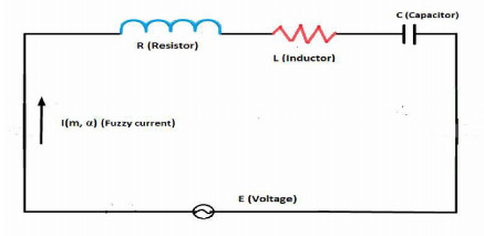
The extraction of analytical solution of uncertain fractional Langevin differential equations involving two independent fractional-order is frequently complex and difficult. As a result, developing a proper and comprehensive technique for the solution of this problem is very essential. In this article, we determine the explicit and analytical fuzzy solution for various classes of the fuzzy fractional Langevin differential equations (FFLDEs) with two independent fractional-orders both in homogeneous and non-homogeneous cases. The potential solution of FFLDEs is also extracted using the fuzzy Laplace transformation technique. Furthermore, the solution of FFLDEs is defined in terms of bivariate and trivariate Mittag-Leffler functions both in the general and special forms. FFLDEs are a new topic having many applications in science and engineering then to grasp the novelty of this work, we connect FFLDEs with RLC electrical circuit to visualize and support the theoretical results.

Keywords:

Citation: Muhammad Akram, Ghulam Muhammad, Tofigh Allahviranloo, Ghada Ali. New analysis of fuzzy fractional Langevin differential equations in Caputo's derivative sense[J]. AIMS Mathematics, 2022, 7(10): 18467-18496. doi: 10.3934/math.20221016

Related Papers:

[1]	Yinwan Cheng, Chao Yang, Bing Yao, Yaqin Luo . Neighbor full sum distinguishing total coloring of Halin graphs. AIMS Mathematics, 2022, 7(4): 6959-6970. doi: 10.3934/math.2022386
[2]	Shabbar Naqvi, Muhammad Salman, Muhammad Ehtisham, Muhammad Fazil, Masood Ur Rehman . On the neighbor-distinguishing in generalized Petersen graphs. AIMS Mathematics, 2021, 6(12): 13734-13745. doi: 10.3934/math.2021797
[3]	Xiaoxue Hu, Jiangxu Kong . An improved upper bound for the dynamic list coloring of 1-planar graphs. AIMS Mathematics, 2022, 7(5): 7337-7348. doi: 10.3934/math.2022409
[4]	Baolin Ma, Chao Yang . Distinguishing colorings of graphs and their subgraphs. AIMS Mathematics, 2023, 8(11): 26561-26573. doi: 10.3934/math.20231357
[5]	Zongpeng Ding . Skewness and the crossing numbers of graphs. AIMS Mathematics, 2023, 8(10): 23989-23996. doi: 10.3934/math.20231223
[6]	Zongrong Qin, Dingjun Lou . The k-subconnectedness of planar graphs. AIMS Mathematics, 2021, 6(6): 5762-5771. doi: 10.3934/math.2021340
[7]	Xin Xu, Xu Zhang, Jiawei Shao . Planar Turán number of double star $S_{3, 4}$ . AIMS Mathematics, 2025, 10(1): 1628-1644. doi: 10.3934/math.2025075
[8]	Yunfeng Tang, Huixin Yin, Miaomiao Han . Star edge coloring of $K_{2, t}$ -free planar graphs. AIMS Mathematics, 2023, 8(6): 13154-13161. doi: 10.3934/math.2023664
[9]	Ana Klobučar Barišić, Antoaneta Klobučar . Double total domination number in certain chemical graphs. AIMS Mathematics, 2022, 7(11): 19629-19640. doi: 10.3934/math.20221076
[10]	Gohar Ali, Martin Bača, Marcela Lascsáková, Andrea Semaničová-Feňovčíková, Ahmad ALoqaily, Nabil Mlaiki . Modular total vertex irregularity strength of graphs. AIMS Mathematics, 2023, 8(4): 7662-7671. doi: 10.3934/math.2023384

Abstract

1. Introduction

Differential equations of arbitrary order have been shown to be useful in the study of models of many phenomena in various fields such as: Electrochemistry and material science, they are in fact described by differential equations of fractional order ^{[9,10,15,16,25,26,27,28,29]}. For more details, we refer the reader to the books of Hilfer ^[30], Podlubny ^[31], Kilbas et al. ^[34], Miller and Ross ^[2] and to the following research papers ^{[1,2,3,4,5,6,7,8,11,12,14,16,17,19,20,24,31,35,36,37,38,39,40,41,42]}. In this work, we discuss the existence and uniqueness of the solutions for multi-point boundary value problems of nonlinear fractional differential equations with two Riemann-Liouville fractionals:

$\begin{equation} \left\{\begin{array}{llll} D^{\alpha}x(t) = \sum^{m}_{i = 1}f_{i}(t, x(t), y(t), \varphi_{1}x(t), \phi_{1}y(t)) , \alpha\in]1, 2], t\in[0, T] &\\ D^{\beta }y(t) = \sum_{i = 1}^{m}g_{i}(t, x(t), y(t), \varphi_{2}x(t), \phi_{2}y(t)) , \beta\in]1, 2], t\in[0, T]& \\ I^{2-\alpha}x(0) = 0, \ D^{\alpha-2}x(T) = \theta I^{\alpha-1}(x(\eta)), \ 0 < \eta < T, &\\ I^{2-\beta}y(0) = 0, \ D^{\beta-2}x(T) = \omega I^{\beta-1}(x(\gamma)), \ 0 < \gamma < T, & \end{array}\right. \end{equation}$

(1.1)

where $D^{(.)}$ , $I^{(.)}$ denote the Riemann-Liouville derivative and integral of fractional order $(.)$ , respectively, $f_{i},$ $g_{i}:\left[0, T\right] \times \mathbb{R}^{4}\rightarrow \mathbb{R},$ $i = 1, \cdots, m$ are continuous functions on $[0, T]$ and

$(\varphi_{1}x)(t) = \int_{0}^{t}A_{1}'(t, s)x(s)ds, \ (\phi_{1}y)(t) = \int_{0}^{t}B_{1}'(t, s)y(s)ds,$

$(\varphi_{2}x)(t) = \int_{0}^{t}A_{2}'(t, s)x(s)ds, \ (\phi_{1}y)(t) = \int_{0}^{t}B_{2}'(t, s)y(s)ds,$

with $A_{i}$ and $B_{i}$ being continuous functions on $[0, 1]\times[0, 1].$ However, it is rare to find a work in nonlinear term $f_{i}$ depends on fractional derivative of unknown functions $x(t), y(t), \varphi_{1}x(t), \phi_{1}y(t)$ and solutions for multi-order fractional differential equations on the infinite interval $[0, T)$ . Motivated by ^{[8,11,12,13,14]} and the references therein, we consider the existence and unicity of solution for multi-order fractional differential equations on infinite interval $[0, T)$ .

The rest of this paper is organized as follow. In section 2, we present some preliminaries and lemmas. Section 3 is dedicated to showing the existence of a solution for problem (1.1). Finally, section 4 illustrated the proposed results with two examples.

Remark 1.1. This work generalizes the work of Houas and Benbachir ^[14] on different boundary conditions and for another type of integral.

2. Preliminaries

This section covers the basic concepts of Riemann-Liouville type fractional calculus that will be used throughout this paper.

Definition 2.1. ^[31,32] The Riemann-Liouville fractional integral operator of order $\alpha \geq 0,$ of a function $f:\left(0, \infty \right) \rightarrow \mathbb{R}$ is defined as

$\begin{eqnarray*} \left\{\begin{array}{ll} J^{\alpha }f\left( t\right) = \frac{1}{\Gamma \left( \alpha \right) }\int_{0}^{t}\left( t-\tau \right) ^{\alpha -1}f\left( \tau \right) d\tau , & \\ J^{0}f\left( t\right) = f\left( t\right) , & \end{array}\right. \end{eqnarray*}$

where $\Gamma \left(\alpha \right) : = \int_{0}^{\infty }e^{-u}u^{\alpha -1}du.$

Definition 2.2. ^[31,32] The Riemann-Liouville fractional derivative of order $\alpha > 0,$ of a continuous function $h:\left(0, \infty \right) \rightarrow \mathbb{R}$ is defined as

$\begin{equation*} D^{\alpha}h\left( t\right) = \frac{1}{\Gamma \left( n-\alpha \right) } \left( \frac{d}{dt}\right) ^{n}\int_{0}^{t}\left( t-\tau \right) ^{n-\alpha-1}h\left( \tau \right) d\tau = \left(\dfrac{d}{dt}\right)^{n}I^{n-\alpha}h(\tau), \end{equation*}$

where $n = \left[\alpha \right] +1.$

For $\alpha < 0$ , we use the convention that $D^{\alpha }h = J^{-\alpha}h.$ Also for $0\leq \rho < \alpha$ , it is valid that $D^{\rho }J^{\alpha }h = h^{\alpha -\rho }.$ We note that for $\varepsilon > -1$ and $\varepsilon \neq \alpha -1, \alpha-2, ..., \alpha-n,$ we have

$\begin{eqnarray*} D^{\alpha}t^{\varepsilon } & = &\frac{\Gamma \left( \varepsilon +1\right) }{\Gamma \left( \varepsilon -\alpha +1\right) }t^{\varepsilon -\alpha }, \\ D^{\alpha}t^{\alpha -i} & = &0, \text{ }i = 1, 2, ..., n. \end{eqnarray*}$

In particular, for the constant function $h(t) = 1$ , we obtain

$D^{\alpha}1 = \dfrac{1}{\Gamma(1-\alpha)}t^{-\alpha}, \alpha\notin\mathbb{N}.$

For $\alpha\in\mathbb{N}$ , we obtain, of course, $D^{\alpha}1 = 0$ because of the poles of the gamma function at the points $0, -1, -2, ...$ For $\alpha > 0$ , the general solution of the homgeneous equation $D^{\alpha}h(t) = 0$ in $C(0, T)\cap L(0, T)$ is

$h(t) = c_{0}t^{\alpha-n}+c_{1}t^{\alpha-n-1}+......+c_{n-2}t^{\alpha-2}+c_{n-1}t^{\alpha-1},$

where $c_{i}, i = 1, 2, ...., n-1$ , are arbitrary real constants. Further, we always have $D^{\alpha}I^{\alpha}h = h$ , and

$D^{\alpha}I^{\alpha}h(t) = h(t)+c_{0}t^{\alpha-n}+c_{1}t^{\alpha-n-1}+......+c_{n-2}t^{\alpha-2}+c_{n-1}t^{\alpha-1}.$

Lemma 2.1. ^[33] Let $E$ be Banach space. Assume that $T : E\longrightarrow E$ is a completely continuous operator. If the set $V = \{x \in E : x = \mu T x, \ 0 < \mu < 1\}$ is bounded, then $T$ has a fixed point in $E$ .

To define the solution for problem (1.1). We consider the following lemma.

Lemma 2.2. Suppose that $(H_{i})_{i = 1, \ldots, m}\subset C([0, 1], \mathbb{R})$ , and consider the problem

$\begin{equation} D^{\alpha}h(t)-\sum\limits_{i = 1}^{m}H_{i}(t) = 0, \ t\in j, \ 1 < \alpha < 2, \ m\in\mathbb{N}^{\ast}, \end{equation}$

(2.1)

with the conditions

$\begin{equation} I^{2-\alpha}h(0) = 0, \ D^{\alpha-2}h(T) = \theta I^{\alpha-1}(h(\eta)), \ 0 < \eta < T. \end{equation}$

(2.2)

Then we have

$\begin{eqnarray*} h(t)& = &\dfrac{1}{\Gamma(\alpha)}\sum\limits_{i = 1}^{m}\int^{t}_{0}(t-\tau)^{\alpha-1}H_{i}(\tau)d\tau\\ &&+\dfrac{t^{\alpha-1}}{\psi}\left(\sum\limits_{i = 1}^{m}\int^{T}_{0}(T-\tau)H_{i}(\tau)d\tau \right. \left. -\dfrac{\theta}{\Gamma(2\alpha)}\sum\limits_{i = 1}^{m}\int^{\eta}_{0}(\eta-\tau)^{2\alpha-2}H_{i}(\tau)d\tau\right) \end{eqnarray*}$

with $\psi = \theta\dfrac{\Gamma(\alpha)}{\Gamma(2\alpha-1)}\eta^{2\alpha-2}-\Gamma(\alpha)T.$

Proof. We have

$h(t) = \sum\limits_{i = 1}^{m}I^{\alpha}H_{i}(t)+c_{0}t^{\alpha-2}+c_{1}t^{\alpha-1},$

where $c_{i}\in\mathbb{R}, \ i = 0, 1.$

We obtain

$\begin{eqnarray*} I^{2-\alpha}h(\tau)& = &\sum\limits_{i = 1}^{m}I^{2}H_{i}(\tau)+c_{0}I^{2-\alpha}\tau^{\alpha-2}+c_{1}I^{2-\alpha}\tau^{\alpha-1}\\ & = &\sum\limits_{i = 1}^{m}I^{2}H_{i}(\tau)+c_{0}+c_{1}\tau , \\ I^{\alpha-1}h(\tau)& = &\sum\limits_{i = 1}^{m}I^{2\alpha-1}H_{i}(\tau)+c_{0}I^{\alpha-1}\tau^{\alpha-2}+c_{1}I^{\alpha-1}\tau^{\alpha-1}\\ & = &\sum\limits_{i = 1}^{m}I^{2\alpha-1}H_{i}(\tau)+c_{0}\dfrac{\Gamma(\alpha-1)}{\Gamma(2\alpha-2)}\tau^{2\alpha-3}+c_{1}\dfrac{\Gamma(\alpha)}{\Gamma(2\alpha-1)}\tau^{2\alpha-2}, \\ D^{\alpha-2}h(\tau)& = &\sum\limits_{i = 1}^{m}I^{2}H_{i}(\tau)+c_{0}\Gamma(\alpha-1)+c_{1}\Gamma(\alpha)\tau. \end{eqnarray*}$

Using the given conditions: $I^{2-\alpha}h(0) = 0$ , we find that $c_{0} = 0$ , and since $D^{\alpha-2}h(T)-\theta I^{\alpha-1}(h(\eta)) = 0$ , we have

$\begin{equation*} \sum\limits_{i = 1}^{m}I^{2}h_{i}(T)+c_{1}\Gamma(\alpha)T-\theta\left[\sum\limits_{i = 1}^{m}I^{2\alpha-1}h_{i}(\eta)+c_{1}\dfrac{\Gamma(\alpha)}{\Gamma(2\alpha-1)}\eta^{2\alpha-2}\right] = 0, \end{equation*}$

then

$\begin{equation*} c_{1}\left[\dfrac{\Gamma(\alpha)}{\Gamma(2\alpha-1)}\eta^{2\alpha-2}-\Gamma(\alpha)T\right] = \sum\limits_{i = 1}^{m}I^{2}h_{i}(T)-\theta\sum\limits_{i = 1}^{m}I^{2\alpha-1}h_{i}(\eta) \end{equation*}$

and

$\begin{eqnarray*} c_{1}& = &\dfrac{1}{\psi}\left(\sum\limits_{i = 1}^{m}I^{2}H_{i}(T)-\theta\sum\limits_{i = 1}^{m}I^{2\alpha-1}H_{i}(\eta)\right)\\ & = &\dfrac{1}{\psi}\left(\sum\limits_{i = 1}^{m}\int_{0}^{T}(T-\tau)H_{i}(\tau)d\tau-\dfrac{\theta}{\Gamma(2\alpha)}\sum\limits_{i = 1}^{m}\int_{0}^{\eta}(\eta-\tau)^{2\alpha-2}H_{i}(\tau)d\tau\right) \end{eqnarray*}$

with

$\begin{eqnarray*} \psi = \theta\dfrac{\Gamma(\alpha)}{\Gamma(2\alpha-1)}\eta^{2\alpha-2}-\Gamma(\alpha)T. \end{eqnarray*}$

Finally, the solution of (2.1) and (2.2) is

$\begin{eqnarray*} h(t)& = &\dfrac{1}{\Gamma(\alpha)}\sum\limits_{i = 1}^{m}\int^{t}_{0}(t-\tau)^{\alpha-1}H_{i}(\tau)d\tau+\dfrac{t^{\alpha-1}}{\psi}\left(\sum\limits_{i = 1}^{m}\int^{T}_{0}(T-\tau)H_{i}(\tau)d\tau \right. \\ &&\qquad \left. -\dfrac{\theta}{\Gamma(2\alpha)}\sum\limits_{i = 1}^{m}\int^{\eta}_{0}(\eta-\tau)^{2\alpha-2}H_{i}(\tau)d\tau\right). \end{eqnarray*}$

3. Main results

We denote by

$E = \{x, y\in C\left( \left[ 0, T\right], \mathbb{R} \right); \varphi_{i}x, \phi_{i}y\in C\left( \left[ 0, T\right], \mathbb{R} \right)\ \ i = 1, 2\},$

and the Banach space of all continuous functions from $\left[0, T \right]$ to $\mathbb{R}$ endowed with a topology of uniform convergence with the norm defined by

$||(x, y)||_{E} = \max\left(||x||, ||y||, ||\varphi_{1} x||, ||\phi_{1}y||, ||\varphi_{2}x||, ||\phi_{2}y||\right),$

where

$\begin{eqnarray*} &&||x|| = \sup\limits_{t\in j}|\varphi_{i}x(t)|, \; \; ||y|| = \sup\limits_{t \in j}|y(t)|, \\ && ||\phi_{i}x|| = \sup\limits_{t\in j}|\varphi_{i}x(t)|, \; \; ||\phi_{i}y|| = \sup\limits_{t \in j}|\phi_{i}y(t)|. \end{eqnarray*}$

In this section, we prove some existence and uniqueness results to the nonlinear fractional coupled system (1.1).

For the sake of convenience, we impose the following hypotheses:

$(H1)$ For each $i = 1, 2, \cdots, m$ , the functions $f_{i}$ and $g_{i}\ \ : [0, T]\times\mathbb{R}^4\longrightarrow\mathbb{R}$ are continuous.

$(H2)$ There exist nonnegative real numbers $\xi^{i}_{k}, \varphi^{i}_{k}, k = 1, 2, 3, 4, i = 1, 2, \cdots, m$ , such that for all $t\in \left[0, T\right]$ and all $(x_{1}, x_{2}, x_{3}, x_{4}),$ $(y_{1}, y_{2}, y_{3}, y_{4})\in \mathbb{R}^{4},$ we have

$\begin{equation*} |f_{i}(t, x_{1}, x_{2}, x_{3}, x_{4})-f_{i}(t, y_{1}, y_{2}, y_{3}, y_{4})|\leq\sum\limits_{k = 1}^{4}\ \xi^{i}_{k} |x_{k}-y_{k}|, \end{equation*}$

and

$\begin{equation*} |g_{i}(t, x_{1}, x_{2}, x_{3}, x_{4})-g_{i}(t, y_{1}, y_{2}, y_{3}, y_{4})|\leq\sum\limits_{k = 1}^{4}\ \chi^{i}_{k} |x_{k}-y_{k}|. \end{equation*}$

$(H3)$ There exist nonnegative constants $(L_{i}) \ \text{and}\ \ (K_{i}) \ i = 1, ..., m$ , such that: For each $t \in [0, T]$ and all $(x_{1}, x_{2}, x_{3}, x_{4}) \in \mathbb{R}^{4},$

$\begin{equation*} | f_{i} (t, x_{1}, x_{2}, x_{3}, x_{4})| \leq L_{i}, |g_{i} (t, x_{1}, x_{2}, x_{3}, x_{4})| \leq K_{i}, i = 1, ..., m. \end{equation*}$

We also consider the following quantities:

$\begin{eqnarray*} A_{1}& = &\dfrac{T^{\alpha}}{\Gamma(\alpha +1)}\sum\limits_{i = 1}^{m}(\xi_{1}^{i}+\xi_{2}^{i}+\xi_{3}^{i}+\xi_{4}^{i}), \\ A_{2}& = &\dfrac{T^{\beta}}{\Gamma(\beta +1)}\sum\limits_{i = 1}^{m}(\chi_{1}^{i}+\chi_{2}^{i}+\chi_{3}^{i}+\chi_{4}^{i}), \\ A_{3}& = &\max\limits_{t, s\in[0, 1]}||A'_{1}(t, s)||\times A_{1}, \\ A_{4}& = &\max\limits_{t, s\in[0, 1]}||A'_{2}(t, s)||\times A_{1}, \\ A_{5}& = &\max\limits_{t, s\in[0, 1]}||B'_{1}(t, s)||\times A_{2}, \\ A_{6}& = &\max\limits_{t, s\in[0, 1]}||B'_{2}(t, s)||\times A_{2}, \\ \nu_{1}& = &\left[\dfrac{T^{\alpha}}{\Gamma(\alpha+1)}+\dfrac{1}{\psi}\left(\dfrac{T^{\alpha+1}}{2}+\dfrac{\theta T^{3\alpha-2}}{(2\alpha-1)^{2}\Gamma(2\alpha-1)}\right)\right], \\ \nu_{2}& = &\left[\dfrac{T^{\beta}}{\Gamma(\beta+1)}+\dfrac{1}{\psi'}\left(\dfrac{T^{\beta+1}}{2}+\dfrac{\omega T^{3\beta-2}}{(2\beta-1)^{2}\Gamma(2\beta-1)}\right)\right], \\ \nu_{3}& = &\max\limits_{t, s\in[0, 1]}|A'_{1}(t, s)|\nu_{1}, \\ \nu_{4}& = &\max\limits_{t, s\in[0, 1]}|A'_{2}(t, s)|\nu_{1}, \\ \nu_{5}& = &\max\limits_{t, s\in[0, 1]}|B'_{1}(t, s)|\nu_{2}, \\ \nu_{6}& = &\max\limits_{t, s\in[0, 1]}|B'_{2}(t, s)|\nu_{2}. \end{eqnarray*}$

3.1. Existence of solutions

The first result is based on Banach contraction principle. We have

Theorem 3.1. Assume that $(H2)$ holds. If the inequality

$\begin{equation} \max(A_{1}, A_{2}, A_{3}, A_{4}, A_{5}, A_{6}) < 1, \end{equation}$

(3.1)

is valid, then the system (1.1) has a unique solution on $[0, T]$ .

Proof. We define the operator $T : E\longrightarrow E$ by

$T(x, y)(t) = (T_{1}(x, y)(t) , T_{2} (x, y)(t)) , t \in[0, T],$

such that

$\begin{eqnarray} T_{1}(x, y)(t)& = &\dfrac{1}{\Gamma(\alpha)}\sum\limits_{i = 1}^{m}\int^{t}_{0}(t-\tau)^{\alpha-1}H_{i}(\tau)d\tau+\dfrac{t^{\alpha-1}}{\psi}\left(\sum\limits_{i = 1}^{m}\int^{T}_{0}(T-\tau)H_{i}(\tau)d\tau \right.\\ &&\qquad \left. -\dfrac{\theta}{\Gamma(2\alpha)}\sum\limits_{i = 1}^{m}\int^{\eta}_{0}(\eta-\tau)^{2\alpha-2}H_{i}(\tau)d\tau\right) \end{eqnarray}$

(3.2)

and

$\begin{eqnarray} T_{2}(x, y)(t)& = &\dfrac{1}{\Gamma(\beta)}\sum\limits_{i = 1}^{m}\int^{t}_{0}(t-\tau)^{\beta-1}G_{i}(\tau)d\tau+\dfrac{t^{\beta-1}}{\psi'}\left(\sum\limits_{i = 1}^{m}\int^{T}_{0}(T-\tau)G_{i}(\tau)d\tau \right.\\ &&\qquad \left. -\dfrac{\omega}{\Gamma(2\beta)}\sum\limits_{i = 1}^{m}\int^{\gamma}_{0}(\gamma-\tau)^{2\beta-2}G_{i}(\tau)d\tau\right) \end{eqnarray}$

(3.3)

where

$H_{i}(\tau) = f_{i}(\tau, x(\tau), y(\tau), \varphi_{1}x(\tau), \phi_{1}y(\tau))$

and

$G_{i}(\tau) = g_{i}(\tau, x(\tau), y(\tau), \varphi_{2}x(\tau), \phi_{2}y(\tau)).$

We obtain

$\varphi_{i} T_{1}(x, y)(t) = \int^{t}_{0}A_{i}(t, s)T_{1}(x, y)(s)ds, \ \phi_{i}T_{2}(x, y)(t) = \int^{t}_{0}B_{i}(t, s)T_{2}(x, y)(s)ds$

where $i = 1, 2.$

We shall now prove that T is contractive.

Let $T_{1}(x_{1}, y_{1}), T_{2} (x_{2}, y_{2})\in E$ . Then, for each $t\in [0, T]$ , we have

$\begin{eqnarray} |T_{1}(x_{1}, y_{1})-T_{1}(x_{2}, y_{2})|&\leq &\left[\dfrac{1}{\Gamma(\alpha)}\sum\limits_{i = 1}^{m}\int^{t}_{0}(t-\tau)^{\alpha-1}d\tau+\dfrac{t^{\alpha-1}}{\psi}\left(\sum\limits_{i = 1}^{m}\int^{T}_{0}(T-\tau)d\tau \right.\right. \\ &&\qquad \left.\left. -\dfrac{\theta}{\Gamma(2\alpha)}\sum\limits_{i = 1}^{m}\int^{\eta}_{0}(\eta-\tau)^{2\alpha-2}d\tau\right)\right]\\ &&\times\max\limits_{\tau\in[0, T]}\sum\limits_{i = 1}^{m} \left|\left(\begin{array}{ll} f_{i}(\tau, x_{1}(\tau), y_{1}(\tau), \varphi_{1}x_{1}(\tau), \phi_{1}y_{1}(\tau))& \\ -f_{i}(\tau, x_{2}(\tau), y_{2}(\tau), \varphi_{1}x_{2}(\tau), \phi_{1}y_{2}(\tau)) & \end{array}\right)\right|\\ &\leq &\dfrac{T^{\alpha}}{\Gamma(\alpha +1)}\max\limits_{\tau\in[0, T]}\sum\limits_{i = 1}^{m} \left|\left(\begin{array}{ll} f_{i}(\tau, x_{1}(\tau), y_{1}(\tau), \varphi_{1}x_{1}(\tau), \phi_{1}y_{1}(\tau)) & \\ -f_{i}(\tau, x_{2}(\tau), y_{2}(\tau), \varphi_{1}x_{2}(\tau), \phi_{1}y_{2}(\tau)) \end{array}\right)\right|. \end{eqnarray}$

By $(H2)$ , it follows that

$\begin{eqnarray*} ||T_{1}(x_{1}, y_{1})-T_{1}(x_{2}, y_{2})||&\leq &\dfrac{T^{\alpha}}{\Gamma(\alpha +1)}\sum\limits_{i = 1}^{m}(\xi_{1}^{i}+\xi_{2}^{i}+\xi_{3}^{i}+\xi_{4}^{i})\times\max(||x_{1}-x_{2}||, ||y_{1}-y_{2}||, \\ &&||\varphi_{1}(x_{1}-x_{2})||, ||\varphi_{2}(x_{1}-x_{2})||, ||\phi_{1}(y_{1}-y_{2})||, ||\phi_{2}(y_{1}-y_{2})||). \end{eqnarray*}$

Hence,

$\begin{equation} ||T_{1}(x_{1}, y_{1})-T_{1}(x_{2}, y_{2})||\leq A_{1}||x_{1}-x_{2}, y_{1}-y_{2}||_{E}. \end{equation}$

(3.4)

With the same arguments as before, we can show that

$\begin{equation} ||T_{2}(x_{1}, y_{1})-T_{2}(x_{2}, y_{2})||\leq A_{2}||x_{1}-x_{2}, y_{1}-y_{2}||_{E}. \end{equation}$

(3.5)

On the other hand, we have

$\begin{eqnarray*} ||\varphi_{1}(T_{1}(x_{1}, y_{1})-T_{1}(x_{2}, y_{2}))||&\leq &\int_{0}^{t}||A'_{1}(t, s)||||T_{1}(x_{1}, y_{1})-T_{1}(x_{2}, y_{2})||ds\\ &\leq &\max\limits_{t, s\in[0, 1]}||A'_{1}(t, s)||\times A_{1}||x_{1}-x_{2}, y_{1}-y_{2}||_{E}. \end{eqnarray*}$

Hence,

$\begin{equation} ||\varphi_{1}(T_{1}(x_{1}, y_{1})-T_{1}(x_{2}, y_{2}))||\leq A_{3}||x_{1}-x_{2}, y_{1}-y_{2}||_{E} \end{equation}$

(3.6)

and

$\begin{equation} ||\varphi_{2}(T_{1}(x_{1}, y_{1})-T_{1}(x_{2}, y_{2}))||\leq A_{4}||x_{1}-x_{2}, y_{1}-y_{2}||_{E}. \end{equation}$

(3.7)

Also, we have

$\begin{equation} ||\phi_{1}(T_{2}(x_{1}, y_{1})-T_{2}(x_{2}, y_{2}))||\leq A_{5}||x_{1}-x_{2}, y_{1}-y_{2}||_{E} \end{equation}$

(3.8)

and

$\begin{equation} ||\phi_{2}(T_{2}(x_{1}, y_{1})-T_{2}(x_{2}, y_{2}))||\leq A_{6}||x_{1}-x_{2}, y_{1}-y_{2}||_{E}. \end{equation}$

(3.9)

Thanks to (3.4)–(3.9), we get

$\begin{eqnarray} ||T(x_{1}, y_{1})-T(x_{2}, y_{2})|| & \leq \max(A_{1}, A_{2}, A_{3}, A_{4}, A_{5}, A_{6})\\ & \times ||(x_{1}-x_{2}, y_{1}-y_{2})||_{E}. \end{eqnarray}$

(3.10)

Thanks to (3.10), we conclude that T is a contractive operator. Therefore, by Banach fixed point theorem, $T$ has a unique fixed point which is the solution of the system (1.1).

3.2. Uniqueness of solutions

Our second main result is based on Lemma 2.1. We have

Theorem 3.2. Assume that the hypotheses $(H1)$ and $(H3)$ are satisfied. Then, system (1.1) has at least a solution on $[0, T]$ .

Proof. The operator $T$ is continuous on $E$ in view of the continuity of $f_{i}$ and $g_{i}$ (hypothesis ( $H1$ )).

Now, we show that $T$ is completely continuous:

(i) First, we prove that $T$ maps bounded sets of $E$ into bounded sets of $E$ . Taking $\lambda > 0$ , and $(x, y)\in \Omega_{\lambda} = \{(x, y) \in E; ||(x, y)||\leq\lambda\}$ , then for each $t\in [0, T]$ , we have:

$\begin{eqnarray*} |T_{1}(x, y)|&\leq &\left[\dfrac{1}{\Gamma(\alpha)}\int^{t}_{0}(t-\tau)^{\alpha-1}d\tau+\dfrac{t^{\alpha-1}}{\psi}\left(\int^{T}_{0}(T-\tau)d\tau \right.\right. \\ \nonumber &&\qquad \left.\left. -\dfrac{\theta}{\Gamma(2\alpha)}\int^{\eta}_{0}(\eta-\tau)^{2\alpha-2}d\tau\right)\right]\\ &&\times\sup\limits_{t\in[0, T]}\sum\limits_{i = 1}^{m} |f_{i}(t, x(t), y(t), \varphi_{1}x(t), \phi_{1}y(t))|\\ &\leq & \left[\dfrac{T^{\alpha}}{\Gamma(\alpha+1)}+\dfrac{1}{\psi}\left(\dfrac{T^{\alpha+1}}{2}+\dfrac{\theta T^{3\alpha-2}}{(2\alpha-1)^{2}\Gamma(2\alpha-1)}\right)\right] \\ &&\times\sup\limits_{t\in[0, T]}\sum\limits_{i = 1}^{m} |f_{i}(t, x(t), y(t), \varphi_{1}x(t), \phi_{1}y(t))|, \end{eqnarray*}$

Thanks to ( $H3$ ), we can write

$||T_{1}(x, y)||\leq\left[\dfrac{T^{\alpha}}{\Gamma(\alpha+1)}+\dfrac{1}{\psi}\left(\dfrac{T^{\alpha+1}}{2}+\dfrac{\theta T^{3\alpha-2}}{(2\alpha-1)^{2}\Gamma(2\alpha-1)}\right)\right]\sum\limits_{i = 1}^{m} L_{i}.$

Thus,

$\begin{equation} ||T_{1}(x, y)||\leq \nu_{1} \sum\limits_{i = 1}^{m} L_{i}. \end{equation}$

(3.11)

As before, we have

$\begin{equation} ||T_{2}(x, y)||\leq \nu_{2} \sum\limits_{i = 1}^{m} K_{i}. \end{equation}$

(3.12)

On the other hand, for all $j = 1, 2$ , we get

$\begin{eqnarray*} |\phi_{j}T_{1}(x, y)(t)| = \left|\int_{0}^{t}A'_{j}(t, s)T_{1}(x, y)(s)ds\right| \leq \max\limits_{t, s\in[0, 1]}|A'_{j}(t, s)|\nu_{1}\sum\limits_{i = 1}^{m} L_{i}. \end{eqnarray*}$

This implies that

$\begin{eqnarray} ||\phi_{1}T_{1}(x, y)(t)||&\leq &\nu_{3}\sum\limits_{i = 1}^{m} L_{i}, \end{eqnarray}$

(3.13)

$\begin{eqnarray} ||\phi_{2}T_{1}(x, y)(t)||&\leq &\nu_{4}\sum\limits_{i = 1}^{m} L_{i}. \end{eqnarray}$

(3.14)

Similarly, we have

$\begin{eqnarray} ||\varphi_{1}T_{2}(x, y)(t)||&\leq &\nu_{5}\sum\limits_{i = 1}^{m} K_{i}, \end{eqnarray}$

(3.15)

$\begin{eqnarray} ||\varphi_{2}T_{2}(x, y)(t)||&\leq &\nu_{6}\sum\limits_{i = 1}^{m} K_{i}. \end{eqnarray}$

(3.16)

It follows from (3.11)–(3.16) that:

$\begin{eqnarray*} ||T(x, y)||_{E}\leq \max \left(\begin{array}{ll} \nu_{1} \sum\limits_{i = 1}^{m} L_{i}, \nu_{2} \sum\limits_{i = 1}^{m} K_{i}, \nu_{3}\sum\limits_{i = 1}^{m} L_{i}, &\\ \nu_{4}\sum\limits_{i = 1}^{m} L_{i}, , \nu_{5}\sum\limits_{i = 1}^{m}, \nu_{6}\sum\limits_{i = 1}^{m}& \end{array}\right). \end{eqnarray*}$

Thus,

$||T(x, y)||_{E} < \infty.$

(ii) Second, we prove that $T$ is equi-continuous:

For any $0 \leq t_{1} < t_{2} \leq T$ and $(x, y) \in\Omega_{\lambda}$ , we have

$\begin{eqnarray*} &&|T_{1}(x, y)(t_{2})-T_{1}(x, y)(t_{1})|\\ &&\qquad\leq \left[\dfrac{1}{\Gamma(\alpha)}\int^{t_{1}}_{0}(t_{2}-\tau)^{\alpha-1}-(t_{1}-\tau)^{\alpha-1}d\tau+\dfrac{1}{\Gamma(\alpha)}\int^{t_{2}}_{t_{1}}(t_{2}-\tau)^{\alpha-1}d\tau\right. \\ &&\qquad\quad\left.+\dfrac{t_{2}^{\alpha-1}-t_{1}^{\alpha-1}}{\psi}\left(\dfrac{T^{2}}{2}-\dfrac{\theta\eta^{2\alpha-1}}{\Gamma(2\alpha-1)^{2}\Gamma(2\alpha-1)}\right)\right]\\ &&\qquad\times\sup\limits_{t\in[0, T]}\sum\limits_{i = 1}^{m} |f_{i}(t, x(t), y(t), \varphi_{1}x(t), \phi_{1}y(t))|\\ &&\qquad\leq\left[\dfrac{2}{\Gamma(\alpha+1)}(t_{2}-t_{1})^{\alpha-1}+(t_{2}^{\alpha-1}-t_{1}^{\alpha-1})\left[\dfrac{T^{2}}{2\psi}\right.\right.\\ &&\qquad\quad\left.\left.-\dfrac{\theta\eta^{2\alpha-1}}{\psi\Gamma(2\alpha-1)^{2}\Gamma(2\alpha-1)}+\dfrac{1}{\Gamma(\alpha+1)}\right]\right]\times\sum\limits_{i = 1}^{m}L_{i}. \end{eqnarray*}$

Therefore,

$\begin{eqnarray} &&||T_{1}(x, y)(t_{2})-T_{1}(x, y)(t_{1})||_{E} \\ &&\quad\left[\dfrac{2}{\Gamma(\alpha+1)}(t_{2}-t_{1})^{\alpha-1}+(t_{2}^{\alpha-1}-t_{1}^{\alpha-1})\left[\dfrac{T^{2}}{2\psi}+\dfrac{1}{\Gamma(\alpha+1)}\right]\right]\times\sum\limits_{i = 1}^{m}L_{i}. \end{eqnarray}$

(3.17)

We also have

$\begin{eqnarray} &&||T_{2}(x, y)(t_{2})-T_{2}(x, y)(t_{1})||_{E} \\ &&\quad\left[\dfrac{2}{\Gamma(\beta+1)}(t_{2}-t_{1})^{\beta-1}+(t_{2}^{\beta-1}-t_{1}^{\beta-1})\left[\dfrac{T^{2}}{2\psi'}+\dfrac{1}{\Gamma(\beta+1)}\right]\right]\times\sum\limits_{i = 1}^{m}K_{i}. \end{eqnarray}$

(3.18)

On the other hand,

$\begin{eqnarray*} &&|\phi_{i}T_{1}(x, y)(t_{2})-\phi_{i}T_{1}(x, y)(t_{1})|\\ &&\quad\leq\left[\max\limits_{s\in[0, 1]}|A_{i}'(t_{2}, s)-A_{i}'(t_{1}, s)|+(t_{2}-t_{1})\max\limits_{s\in[0, 1]}|A_{i}'(t_{1}, s)|\right] \times\sup\limits_{s\in[0, 1]}|T_{1}(x, y)(s)|. \end{eqnarray*}$

Consequently, for all $i = 1, 2,$ we obtain

$\begin{eqnarray} &&||\phi_{i}T_{1}(x, y)(t_{2})-\phi_{i}T_{1}(x, y)(t_{1})||\\ &&\quad\leq\left[\max\limits_{s\in[0, 1]}|A_{i}'(t_{2}, s)-A_{i}'(t_{1}, s)|+(t_{2}-t_{1})\max\limits_{s\in[0, 1]}|A_{i}'(t_{1}, s)|\right] \nu_{1}\sum\limits_{i = 1}^{m}L_{i}. \end{eqnarray}$

(3.19)

Similarly,

$\begin{eqnarray} &&||\varphi_{i}T_{1}(x, y)(t_{2})-\varphi_{i}T_{1}(x, y)(t_{1})||\\ &&\quad\leq\left[\max\limits_{s\in[0, 1]}|B_{i}'(t_{2}, s)-B_{i}'(t_{1}, s)|+(t_{2}-t_{1})\max\limits_{s\in[0, 1]}|B_{i}'(t_{1}, s)|\right] \nu_{2}\sum\limits_{i = 1}^{m}K_{i}. \end{eqnarray}$

(3.20)

where $i = 1, 2$ . Using (3.17)–(3.20), we deduce that

$||T(x, y)(t_{2})-T(x, y)(t_{1})||_{E}\longrightarrow 0$

as $t_{2}\rightarrow t_{1}.$

Combining (i) and (ii), we conclude that $T$ is completely continuous.

(iii) Finally, we shall prove that the set $F$ defined by

$F = \{(x, y) \in E, (x, y) = \rho T (x, y), \ 0 < \rho < 1 \}$

is bounded.

Let $(x, y)\in F$ , then $(x, y) = \rho T (x, y)$ , for some $0 < \rho < 1$ . Thus, for each $t \in [0, T]$ , we have:

$\begin{equation} x(t) = \rho T_{1}(x, y)(t), \ y (t) = \rho T_{2}(x, y)(t) . \end{equation}$

(3.21)

Thanks to ( $H3$ ) and using (3.11) and (3.12), we deduce that

$\begin{equation} ||x||\leq\rho\nu_{1}\sum\limits_{i = 1}^{m}L_{i}, \ ||y|| \leq\rho\nu_{2} \sum\limits_{i = 1}^{m}K_{i} . \end{equation}$

(3.22)

Using (3.13)–(3.16), it yields that

$\begin{eqnarray} \left\{\begin{array}{llll} ||\phi_{1}x||\leq \rho\nu_{3} \sum_{i = 1}^{m}L_{i} & \\ ||\phi_{2}x||\leq \rho\nu_{4} \sum_{i = 1}^{m}L_{i} & \\ ||\varphi_{1}y||\leq \rho\nu_{5} \sum_{i = 1}^{m}K_{i} & \\ ||\varphi_{2}y||\leq \rho\nu_{6} \sum_{i = 1}^{m}K_{i} & \end{array}\right.. \end{eqnarray}$

(3.23)

It follows from (3.22) and (3.23) that

$\begin{eqnarray*} ||T(x, y)||_{E}\leq \rho\max \left(\begin{array}{ll} \nu_{1} \sum_{i = 1}^{m} L_{i}, \nu_{2} \sum_{i = 1}^{m} K_{i}, \nu_{3}\sum_{i = 1}^{m} L_{i}, &\\ \nu_{4}\sum_{i = 1}^{m} L_{i}, , \nu_{5}\sum_{i = 1}^{m}, \nu_{6}\sum_{i = 1}^{m}& \end{array}\right). \end{eqnarray*}$

Consequently,

$||(x, y)||_{E} < \infty.$

This shows that $F$ is bounded. By Lemma (2.1), we deduce that $T$ has a fixed point, which is a solution of (1.1).

4. Related examples

To illustrate our main results, we treat the following examples.

Example 4.1. Consider the following system:

$\begin{eqnarray} \left\{\begin{array}{llllll} D^{\frac{3}{2}}x(t) = \dfrac{\cos(\pi t)(x+y+\varphi_{1}x(t)+\phi_{1}y(t))}{10\pi(x+y+\varphi_{1}x(t)+\phi_{1}y(t))}+\dfrac{1}{32\pi^{2}e}&\\ \\ \qquad\qquad\qquad \left(\cos x(t)+\cos y(t)+\dfrac{\varphi_{1}x(t)+\phi_{1}y(t)}{4\pi}\right), &\\ \\ D^{\frac{3}{2}}y(t) = \dfrac{1}{8\pi^{3}(t+1)}\left(\dfrac{x+y+\varphi_{2}x(t)+\phi_{2}y(t)}{3+x+y+\varphi_{2}x(t)+\phi_{2}y(t)}\right)+\dfrac{1}{(10\pi+e^{t})e^{(t+1)}}&\\ \\ \qquad\qquad\qquad \left(\dfrac{\sin x(t)+\sin y(t)+\cos\varphi_{2}x(t)+\cos\phi_{2}y(t) }{2+\sin x(t)+\sin y(t)+\cos\varphi_{2}x(t)+\cos\phi_{2}y(t)}\right), \\ \\ I^{\frac{1}{2}}x(0) = 0, \ D^{-\frac{1}{2}}x(T) = I^{\frac{1}{2}}(x(1)), &\\ I^{\frac{1}{2}}y(0) = 0, \ D^{-\frac{1}{2}}y(T) = I^{\frac{1}{2}}(y(1)).& \end{array}\right. \end{eqnarray}$

(4.1)

We have

$\alpha = \dfrac{3}{2}, \ \beta = \dfrac{3}{2}, \ T = 1, \ \theta = 1, \ \omega = 1, \ \gamma = 1, \ m = 2, \ \eta = 1.$

Also,

$\begin{eqnarray} f_{1}(t, x(t), y(t), \varphi_{1}x(t), \phi_{1}y(t))& = & \dfrac{\cos(\pi t)(x+y+\varphi_{1}x(t)+\phi_{1}y(t))}{10\pi(1+x+y+\varphi_{1}x(t)+\phi_{1}y(t))}, \end{eqnarray}$

(4.2)

$\begin{eqnarray} f_{2}(t, x(t), y(t), \varphi_{1}x(t), \phi_{1}y(t))& = &\dfrac{1}{32\pi^{2}e}\left(\cos x(t)+\cos y(t)+\dfrac{\varphi_{1}x(t)+\phi_{1}y(t)}{4\pi}\right).\\ \end{eqnarray}$

(4.3)

For $t \in [0, 1]$ and $(x_{1}, y_{1}, \varphi_{1}x_{1}, \phi_{1}y_{1}), (x_{2}, y_{2}, \varphi_{1}x_{2}, \phi_{1}y_{2})\in\mathbb{R}^{4}$ , we have

$\begin{eqnarray} &&|f_{1}(t, x_{1}, y_{1}, \varphi_{1}x_{1}, \phi_{1}y_{1})-f_{1}(t, x_{2}, y_{2}, \varphi_{1}x_{2}, \phi_{1}y_{2})|\\ &&\leq\dfrac{|\cos(\pi t)|}{10\pi}\left|\dfrac{x_{1}+y_{1}+\varphi_{1}x_{1}+\phi_{1}y_{1}}{1+x_{1}+y_{1}+\varphi_{1}x_{1}+\phi_{1}y_{1}}-\dfrac{x_{2}+y_{2}+\varphi_{1}x_{2}+\phi_{1}y_{2})}{1+x_{2}+y_{2}+\varphi_{1}x_{2}+\phi_{1}y_{2})}\right|\\ &&\leq \dfrac{1}{10\pi}(|x_{1}-x_{2}|+|y_{1}-y_{2}|+|\varphi_{1}x_{1}-\varphi_{1}x_{2}|+|\phi_{1}y_{1}-\phi_{1}y_{2}|) \end{eqnarray}$

(4.4)

and

$\begin{eqnarray} &&|f_{2}(t, x_{1}, y_{1}, \varphi_{1}x_{1}, \phi_{1}y_{1})-f_{2}(t, x_{2}, y_{2}, \varphi_{1}x_{2}, \phi_{1}y_{2})|\\ &&\quad\leq \dfrac{1}{32\pi e}(|x_{1}-x_{2}|+|y_{1}-y_{2}|+|\varphi_{1}x_{1}-\varphi_{1}x_{2}|+|\phi_{1}y_{1}-\phi_{1}y_{2}|). \end{eqnarray}$

(4.5)

So, we can take

$\xi_{1}^{1} = \xi_{2}^{1} = \xi_{3}^{1} = \xi_{4}^{1} = \dfrac{1}{10\pi},$

$\xi_{1}^{2} = \xi_{2}^{2} = \xi_{3}^{2} = \xi_{4}^{2} = \dfrac{1}{32\pi e}.$

We also have

$\begin{eqnarray} g_{1}(t, x(t), y(t), \varphi_{2}x(t), \phi_{2}y(t))& = &\dfrac{1}{8\pi^{3}(t+1)}\left(\dfrac{x+y+\varphi_{2}x(t)+\phi_{2}y(t)}{3+x+y+\varphi_{2}x(t)+\phi_{2}y(t)}\right) \end{eqnarray}$

and

$\begin{eqnarray} && g_{2}(t, x(t), y(t), \varphi_{2}x(t), \phi_{2}y(t))\\ && = \dfrac{1}{(10\pi +e^{t})e^{t+1}} \left(\dfrac{\sin x(t)+\sin y(t)+\cos\varphi_{2}x(t)+\cos\phi_{2}y(t) }{2+\sin x(t)+\sin y(t)+\cos\varphi_{2}x(t)+\cos\phi_{2}y(t)}\right) \end{eqnarray}$

(4.6)

For $t \in [0, 1]$ and $(x_{1}, y_{1}, \varphi_{2}x_{1}, \phi_{2}y_{1}), (x_{2}, y_{2}, \varphi_{2}x_{2}, \phi_{2}y_{2})\in\mathbb{R}^{4}$ , we can write

$\begin{eqnarray} &&|g_{1}(t, x_{1}, y_{1}, \varphi_{2}x_{1}, \phi_{2}y_{1})-g_{1}(t, x_{2}, y_{2}, \varphi_{2}x_{2}, \phi_{2}y_{2})|\\ &&\quad \leq \dfrac{1}{8\pi^{3}}(|x_{1}-x_{2}|+|y_{1}-y_{2}|+|\varphi_{2}x_{1}-\varphi_{2}x_{2}|+|\phi_{2}y_{1}-\phi_{2}y_{2}|), \end{eqnarray}$

(4.7)

and

$\begin{eqnarray} &&|g_{2}(t, x_{1}, y_{1}, \varphi_{2}x_{1}, \phi_{2}y_{1})-g_{2}(t, x_{2}, y_{2}, \varphi_{2}x_{2}, \phi_{2}y_{2})|\\ &&\quad \leq \dfrac{1}{10\pi e^{2}}(|x_{1}-x_{2}|+|y_{1}-y_{2}|+|\varphi_{2}x_{1}-\varphi_{2}x_{2}|+|\phi_{2}y_{1}-\phi_{2}y_{2}|). \end{eqnarray}$

(4.8)

Hence,

$\chi_{1}^{1} = \chi_{2}^{1} = \chi_{3}^{1} = \chi_{4}^{1} = \dfrac{1}{8\pi^{3}},$

$\chi_{1}^{2} = \chi_{2}^{2} = \chi_{3}^{2} = \chi_{4}^{2} = \dfrac{1}{10\pi e^{2}}.$

Therefore,

$A_{1} = 0.0589009676, \; \; A_{2} = 0.0250930393.$

Suppose

$A'_{i} = B'_{i} = 1, \ i = 1, 2,$

so,

$A_{1} = A_{3} = A_{4}, \; \; A_{2} = A_{5} = A_{6}.$

Thus,

$\begin{equation} \max(A_{1}, A_{2}, A_{3}, A_{4}, A_{5}, A_{6}) < 1, \end{equation}$

(4.9)

and by Theorem 3.1, we conclude that the system (4.1) has a unique solution on $[0, 1]$ .

Example 4.2.

$\begin{eqnarray} \left\{\begin{array}{llllll} D^{\frac{3}{2}}x(t) = \dfrac{\pi( t+1)\sin(\varphi_{1}x(t)+\phi_{1}y(t))}{2-\cos(x(t)+y(t))}&\\ \\ \qquad\qquad\qquad +\dfrac{e^{t}}{2\pi+\cos(x(t)+\varphi_{1}x(t))+\sin(\sin(y(t)+\phi_{1}y(t))}, \ t\in[0, 1], &\\ \\ D^{\frac{4}{3}}y(t) = \dfrac{e^{2}\sin(x(t)+y(t))}{2\pi+\cos(\varphi_{2}x(t)+\phi_{2}y(t))}&\\ \\ \qquad\qquad\qquad +\dfrac{3 t^{2}\cos y(t)}{e^{t^{3}+1}-\cos( x(t)+y(t)-\varphi_{2}x(t)-\phi_{2}y(t))}, \ t\in[0, 1], \\ \\ I^{\frac{1}{2}}x(0) = 0, \ D^{-\frac{1}{2}}x(T) = I^{\frac{1}{2}}(x(1)), &\\ I^{\frac{2}{3}}y(0) = 0, \ D^{-\frac{2}{3}}y(T) = I^{\frac{1}{3}}(y(1)).& \end{array}\right. \end{eqnarray}$

(4.10)

We have

$\alpha = \dfrac{3}{2}, \ \beta = \dfrac{4}{3}, \ T = 1, \ \theta = 1, \ \omega = 1, \ \gamma = 1, \ m = 2, \ \eta = 1.$

Since

$\begin{eqnarray} |f_{1}(t, x(t), y(t), \varphi_{1}x(t), \phi_{1}y(t))|& = &\left|\dfrac{\pi( t+1)\sin(\varphi_{1}x(t)+\phi_{1}y(t))}{2-\cos(x(t)+y(t))}\right| \leq 2\pi , \\ |f_{2}(t, x(t), y(t), \varphi_{1}x(t), \phi_{1}y(t))|& = &\left|\dfrac{e^{t}}{2\pi+\cos(x(t)+\varphi_{1}x(t))+\sin(\sin(y(t)+\phi_{1}y(t))}\right| \leq \dfrac{e}{2\pi +2}, \\ |g_{1}(t, x(t), y(t), \varphi_{2}x(t), \phi_{2}y(t))|& = &\left|\dfrac{e^{2}\sin(x(t)+y(t))}{2\pi+\cos(\varphi_{2}x(t)+\phi_{2}y(t))}\right| \leq \dfrac{e^{2}}{2\pi +1}, \\ |g_{2}(t, x(t), y(t), \varphi_{2}x(t), \phi_{2}y(t))|& = &\left|\dfrac{3 t^{2}\cos y(t)}{e^{t^{3}+1}-\cos( x(t)+y(t)-\varphi_{2}x(t)-\phi_{2}y(t))}\right| \leq \dfrac{3}{e-1}. \end{eqnarray}$

The functions $f_{1}, \ f_{2}, \ g_{1}\ \text{and}\ g_{2}$ are continuous and bounded on $[0, 1]\times\mathbb{R}^{4}$ . So, by Theorem 3.2, the system (4.10) has at least one solution on $[0, 1]$ .

5. Conclusions

We have proved the existence of solutions for fractional differential equations with integral and multi-point boundary conditions. The problem is solved by applying some fixed point theorems. We also provide examples to make our results clear.

Conflict of interest

The authors declare that they have no conflicts of interest in this paper.

References

[1]	D. Dubios, H. Prade, Towards fuzzy differential calculus part 3: Differentiation, Fuzzy Set. Syst., 8 (1982), 225–233.
[2]	M. L. Puri, D. A. Ralescu, Differentials of fuzzy functions, J. Math. Anal. Appl., 91 (1983), 552–558. https://doi.org/10.1016/0022-247X(83)90169-5 doi: 10.1016/0022-247X(83)90169-5
[3]	R. G. Jr, W. Voxman, Elementary fuzzy calculus, Fuzzy Set. Syst., 18 (1986), 31–43. https://doi.org/10.1016/0165-0114(86)90026-6 doi: 10.1016/0165-0114(86)90026-6
[4]	S. Seikkala, On the fuzzy initial value problem, Fuzzy Set. Syst., 24 (1987), 319–330. https://doi.org/10.1016/0165-0114(87)90030-3 doi: 10.1016/0165-0114(87)90030-3
[5]	M. Friedman, M. Ming, A. Kandel, Fuzzy derivatives and fuzzy Cauchy problems using LP metric, In Fuzzy Logic Foundations and Industrial Applications, Springer, Boston, 8 (1996), 57–72. https://doi.org/10.1007/978-1-4613-1441-7_3
[6]	Z. Yue, W. Guangyuan, Time domain methods for the solutions of $N$ -order fuzzy differential equations, Fuzzy Set. Syst., 94 (1998), 77–92. https://doi.org/10.1016/S0165-0114(96)00235-7 doi: 10.1016/S0165-0114(96)00235-7
[7]	B. Bede, S. G. Gal, Generalizations of the differentiability of fuzzy-number-valued functions with applications to fuzzy differential equations, Fuzzy Set. Syst., 151 (2005), 581–599. https://doi.org/10.1016/j.fss.2004.08.001 doi: 10.1016/j.fss.2004.08.001
[8]	M. M. Raja, V. Vijayakumar, Optimal control results for Sobolev-type fractional mixed Volterra-Fredholm type integrodifferential equations of order $1 < r < 2$ with sectorial operators, Opt. Contr. Appl. Met., 2022. https://doi.org/10.1002/oca.2892 doi: 10.1002/oca.2892
[9]	M. M. Raja, V. Vijayakumar, A. Shukla, K. S. Nisar, N. Sakthivel, K. Kaliraj, Optimal control and approximate controllability for fractional integrodifferential evolution equations with infinite delay of order $r\in(1, 2)$ , Opt. Contr. Appl. Met., 2022. https://doi.org/10.1002/oca.2867 doi: 10.1002/oca.2867
[10]	Y. K. Ma, M. M. Raja, V. Vijayakumar, A. Shukla, W. Albalawi, K. S. Nisar, Existence and continuous dependence results for fractional evolution integrodifferential equations of order $r\in(1, 2)$ , Alex. Eng. J., 61 (2022), 9929–9939. https://doi.org/10.1016/j.aej.2022.03.010 doi: 10.1016/j.aej.2022.03.010
[11]	Y. K. Ma, M. M. Raja, K. S. Nisar, A. Shukla, V. Vijayakumar, Results on controllability for Sobolev type fractional differential equations of order $1< r< 2$ with finite delay, AIMS Math., 7 (2022), 10215–10233. https://doi.org/10.3934/math.2022568 doi: 10.3934/math.2022568
[12]	M. M. Raja, V. Vijayakumar, A. Shukla, K. S. Nisar, H. M. Baskonus, On the approximate controllability results for fractional integrodifferential systems of order $1< r< 2$ with sectorial operators, J. Comput. Appl. Math., 415 (2022), 114492. https://doi.org/10.1016/j.cam.2022.114492 doi: 10.1016/j.cam.2022.114492
[13]	R. P. Agarwal, V. Lakshmikantham, J. J. Nieto, On the concept of solution for fractional differential equations with uncertainty, Nonlinear Anal.-Theor., 72 (2010), 2859–2862. https://doi.org/10.1016/j.na.2009.11.029 doi: 10.1016/j.na.2009.11.029
[14]	J. U. Jeong, Existence results for fractional order fuzzy differential equations with infinite delay, Int. Math. Forum, 5 (2010), 3221–3230.
[15]	S. Arshad, V. Lupulescu, On the fractional differential equations with uncertainty, Nonlinear Anal.-Theor., 74 (2011), 3685–3693. https://doi.org/10.1016/j.na.2011.02.048 doi: 10.1016/j.na.2011.02.048
[16]	S. Salahshour, T. Allahviranloo, S. Abbasbandy, Solving fuzzy fractional differential equations by fuzzy Laplace transforms, Commun. Nonlinear Sci., 17 (2012), 1372–1381. https://doi.org/10.1016/j.cnsns.2011.07.005 doi: 10.1016/j.cnsns.2011.07.005
[17]	M. Mazandarani, A. V. Kamyad, Modified fractional Euler method for solving fuzzy fractional initial value problem, Commun. Nonlinear Sci., 18 (2013), 12–21. https://doi.org/10.1016/j.cnsns.2012.06.008 doi: 10.1016/j.cnsns.2012.06.008
[18]	S. Salahshour, T. Allahviranloo, S. Abbasbandy, D. Baleanu, Existence and uniqueness results for fractional differential equations with uncertainty, Adv. Differ. Equ., 2012 (2012), 1–12. https://doi.org/10.1186/1687-1847-2012-112 doi: 10.1186/1687-1847-2012-112
[19]	S. Arshad, On existence and uniqueness of solution of fuzzy fractional differential equations, Iran. J. Fuzzy Syst., 10 (2013), 137–151.
[20]	T. Allahviranloo, A. Armand, Z. Gouyandeh, Fuzzy fractional differential equations under generalized fuzzy Caputo derivative, J. Intell. Fuzzy Syst., 26 (2014), 1481–1490. https://doi.org/10.3233/IFS-130831 doi: 10.3233/IFS-130831
[21]	T. Allahviranloo, Fuzzy fractional differential operators and equations: Fuzzy fractional differential equations, Studies in fuzziness and soft computing series, Springer Nature, Switzerland, 2020. https://doi.org/10.1007/978-3-030-51272-9
[22]	A. Khastan, J. J. Nieto, R. Rodríguez-López, Schauder fixed-point theorem in semilinear spaces and its application to fractional differential equations with uncertainty, Fixed Point Theory A., 2014 (2014), 1–14. https://doi.org/10.1186/1687-1812-2014-21 doi: 10.1186/1687-1812-2014-21
[23]	N. V. Hoa, V. Lupulescu, D. O'Regan, Solving interval-valued fractional initial value problems under Caputo $gH$ -fractional differentiability, Fuzzy Set. Syst., 309 (2017), 1–34. https://doi.org/10.1016/j.fss.2016.09.015 doi: 10.1016/j.fss.2016.09.015
[24]	H. V. Ngo, V. Lupulescu, D. O'Regan, A note on initial value problems for fractional fuzzy differential equations, Fuzzy Set. Syst., 347 (2018), 54–69. https://doi.org/10.1016/j.fss.2017.10.002 doi: 10.1016/j.fss.2017.10.002
[25]	S. Melliani, E. Arhrrabi, M. H. Elomari, L. S. Chadli, Ulam-Hyers-Rassias stability for fuzzy fractional integrodifferential equations under Caputo gH-differentiability, Int. J. Optim. Appl., 2021, 51. https://doi.org/10.1007/s40306-017-0207-2 doi: 10.1007/s40306-017-0207-2
[26]	H. Vu, N. V. Hoa, Uncertain fractional differential equations on a time scale under granular differentiability concept, Comput. Appl. Math., 38 (2019), 1–22. https://doi.org/10.1007/s40314-019-0873-x doi: 10.1007/s40314-019-0873-x
[27]	S. Ezadi, T. Allahviranloo, Artificial neural network approach for solving fuzzy fractional order initial value problems under gH-differentiability, Math. Method. Appl. Sci., 2020. https://doi.org/10.1002/mma.7287 doi: 10.1002/mma.7287
[28]	M. Saqib, M. Akram, S. Bashir, T. Allahviranloo, Numerical solution of bipolar fuzzy initial value problem, J. Intell. Fuzzy Syst., 40 (2021), 1309–1341. https://doi.org/10.3233/JIFS-201619 doi: 10.3233/JIFS-201619
[29]	M. Akram, M. Saqib, S. Bashir, T. Allahviranloo, An efficient numerical method for solving $m$ -polar fuzzy initial value problems, Comput. Appl. Math., 41 (2022), 157. https://doi.org/10.1007/s40314-022-01841-2 doi: 10.1007/s40314-022-01841-2
[30]	M. Akram, M. Ali, T. Allahviranloo, A method for solving bipolar fuzzy complex linear systems with real and complex coefficients, Soft Comput., 26 (2022), 2157–2178. https://doi.org/10.1007/s00500-021-06672-7 doi: 10.1007/s00500-021-06672-7
[31]	M. Akram, T. Allahviranloo, W. Pedrycz, M. Ali, Methods for solving LR-bipolar fuzzy linear systems, Soft Comput., 25 (2021), 85–108. https://doi.org/10.1007/s00500-020-05460-z doi: 10.1007/s00500-020-05460-z
[32]	A. N. A. Koam, M. Akram, G. Muhammad, N. Hussain, LU decomposition scheme for solving m-polar fuzzy system of linear equations, Math. Probl. Eng., 2020 (2020), 8384593. https://doi.org/10.1155/2020/8384593 doi: 10.1155/2020/8384593
[33]	M. Ghaffari, T. Allahviranloo, S. Abbasbandy, M. Azhini, On the fuzzy solutions of time-fractional problems, Iran. J. Fuzzy Syst., 18 (2021), 51–66. https://doi.org/10.22111/IJFS.2021.6081 doi: 10.22111/IJFS.2021.6081
[34]	M. Keshavarz, T. Allahviranloo, Fuzzy fractional diffusion processes and drug release, Fuzzy Set. Syst., 436 (2022), 82–101. https://doi.org/10.1016/j.fss.2021.04.001 doi: 10.1016/j.fss.2021.04.001
[35]	M. Keshavarz, T. Allahviranloo, S. Abbasbandy, M. H. Modarressi, A study of fuzzy methods for solving system of fuzzy differential equations, New Math. Nat. Comput., 17 (2021), 1–27. https://doi.org/10.1142/S1793005721500010 doi: 10.1142/S1793005721500010
[36]	D. Qiu, The generalized Hukuhara differentiability of interval-valued function is not fully equivalent to the one-sided differentiability of its end point functions, Fuzzy Set. Syst., 419 (2021), 158–168. https://doi.org/10.1016/j.fss.2020.07.012 doi: 10.1016/j.fss.2020.07.012
[37]	H. Wang, R. Rodriguez-Lopez, On the existence of solutions to boundary value problems for interval-valued differential equations under gH-differentiability, Inform. Sci., 553 (2021), 225–246. https://doi.org/10.1016/j.ins.2020.10.052 doi: 10.1016/j.ins.2020.10.052
[38]	P. Langevin, Sur la théorie du mouvement brownien, Compt. Rendus, 146 (1908), 530–533.
[39]	M. Z. Ahmad, M. K. Hassan, S. Abbasbanday, Solving fuzzy fractional differential equations using Zadeh's extension principle, The Scientific World J., 2013 (2013). https://doi.org/10.1155/2013/454969 doi: 10.1155/2013/454969
[40]	R. L. Magin, Fractional calculus in bioengineering, Begell House Publisher, Connecticut, 2006. https://doi.org/10.1615/CritRevBiomedEng.v32.i1.10
[41]	T. R. Prabhakar, A singular integral equation with a generalized Mittag-Leffler function in the kernel, Yokohama Math. J., 1971.
[42]	M. Akram, T. Ihsan, T. Allahviranloo, Solving Pythagorean fuzzy fractional differential equations using Laplace transform, Granular Comput., 2022. https://doi.org/10.1007/s41066-022-00344-z doi: 10.1007/s41066-022-00344-z
[43]	D. Baleanu, J. A. T. Machado, A. C. J. Luo, Fractional dynamics and control, Springer Science & Business Media, 2011.
[44]	V. Lakshmikantham, S. Leela, J. V. Devi, Theory of fractional dynamic systems, Cambridge Scientific Publishers, Cambridge, 2009.
[45]	R. Kubo, The fluctuation-dissipation theorem, Rep. Prog. Phys., 29 (1966), 255–284.
[46]	E. Lutz, Fractional Langevin equation, Phys. Rev. E, 64 (2001), 1–4. https://doi.org/10.1142/9789814340595_0012 doi: 10.1142/9789814340595_0012
[47]	Y. Adjabi, M. E. Samei, M. M. Matar, J. Alzabut, Langevin differential equation in frame of ordinary and Hadamard fractional derivatives under three point boundary conditions, AIMS Math., 6 (2021), 2796–2843. https://doi.org/10.3934/math.2021171 doi: 10.3934/math.2021171
[48]	B. Ahmad, A. Alsaedi, S. Salem, On a nonlocal integral boundary value problem of nonlinear Langevin equation with different fractional orders, Adv. Differ. Equ., 2019 (2019), 57. https://doi.org/10.1186/s13662-019-2003-x doi: 10.1186/s13662-019-2003-x
[49]	B. Ahmad, J. J. Nieto, A. Alsaedi, M. El-Shahed, A study of nonlinear Langevin equation involving two fractional orders in different intervals, Nonlinear Anal., 13 (2012), 599–606. https://doi.org/10.1016/j.nonrwa.2011.07.052 doi: 10.1016/j.nonrwa.2011.07.052
[50]	H. Baghani, Existence and uniqueness of solutions to fractional Langevin equations involving two fractional orders, J. Fix. Point Theory A., 20 (2018), 1–7. https://doi.org/10.1007/s11784-018-0540-7 doi: 10.1007/s11784-018-0540-7
[51]	Z. Kiyamehr, H. Baghani, Existence of solutions of BVPs for fractional Langevin equations involving Caputo fractional derivatives, J. Appl. Anal., 27 (2021), 47–55. https://doi.org/10.1515/jaa-2020-2029 doi: 10.1515/jaa-2020-2029
[52]	A. Salem, Existence results of solutions for anti-periodic fractional Langevin equation, J. Appl. Anal. Comput., 10 (2020), 2557–2574. https://doi.org/10.11948/20190419 doi: 10.11948/20190419
[53]	T. Kaczorek, Positive different orders fractional $2$ D linear systems, Acta Mech. Automatica, 2 (2008), 51–58.
[54]	S. S. Devi, K. Ganesan, Modelling electric circuit problem with fuzzy differential equations, J. Phys. Conf. Ser., 1377 (2019), 012024. https://doi.org/10.1088/1742-6596/1377/1/012024 doi: 10.1088/1742-6596/1377/1/012024
[55]	A. Ahmadova, N. I. Mahmudov, Langevin differential equations with general fractional orders and their applications to electric circuit theory, J. Comput. Appl. Math., 388 (2021), 113299. https://doi.org/10.1016/j.cam.2020.113299 doi: 10.1016/j.cam.2020.113299
[56]	K. Diethelm, The analysis of fractional differential equations: An application-oriented exposition using differential operators of Caputo type, Springer, Berlin, 2004.
[57]	I. Podlubny, Fractional differential equations, Academic Press, San Diego, 1999.
[58]	S. G. Samko, A. A. Kilbas, O. I. Marichev, Fractional integrals and derivatives: Theory and applications, Gordon & Breach Science Publishers, Yverdon, 1993.
[59]	A. Fernandez, C. K $\ddot{u}$ rt, M. A. $\ddot{O}$ zarslan, A naturally emerging bivariate Mittag-Leffler function and associated fractional-calculus operators, Comput. Appl. Math., 39 (2020), 1–27. https://doi.org/10.1007/s40314-020-01224-5 doi: 10.1007/s40314-020-01224-5
[60]	A. Ahmadova, I. T. Huseynov, A. Fernandez, N. I. Mahmudov, Trivariate Mittag-Leffler functions used to solve multi-order systems of fractional differential equations, Commun. Nonlinear Sci., 97 (2021), 105735. https://doi.org/10.1016/j.cnsns.2021.105735 doi: 10.1016/j.cnsns.2021.105735
[61]	T. Allahviranloo, M. B. Ahmadi, Fuzzy Laplace transforms, Soft Comput., 14 (2010) 235. https://doi.org/10.1007/s00500-008-0397-6 doi: 10.1007/s00500-008-0397-6

Reader Comments

Your name:*

Email:*
© 2022 the Author(s), licensee AIMS Press. This is an open access article distributed under the terms of the Creative Commons Attribution License (http://creativecommons.org/licenses/by/4.0)