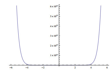
A remarkably large number of polynomials and their extensions have been presented and studied. In the present paper, we introduce the new type of generating function of Appell-type Changhee-Euler polynomials by combining the Appell-type Changhee polynomials and Euler polynomials and the numbers corresponding to these polynomials are also investigated. Certain relations and identities involving these polynomials are established. Further, the differential equations arising from the generating function of the Appell-type Changhee-Euler polynomials are derived. Also, the graphical representations of the zeros of these polynomials are explored for different values of indices.
Citation: Tabinda Nahid, Mohd Saif, Serkan Araci. A new class of Appell-type Changhee-Euler polynomials and related properties[J]. AIMS Mathematics, 2021, 6(12): 13566-13579. doi: 10.3934/math.2021788
A remarkably large number of polynomials and their extensions have been presented and studied. In the present paper, we introduce the new type of generating function of Appell-type Changhee-Euler polynomials by combining the Appell-type Changhee polynomials and Euler polynomials and the numbers corresponding to these polynomials are also investigated. Certain relations and identities involving these polynomials are established. Further, the differential equations arising from the generating function of the Appell-type Changhee-Euler polynomials are derived. Also, the graphical representations of the zeros of these polynomials are explored for different values of indices.

| [1] |
L. Aceto, H. R. Malonek, G. Tomaz, A unified matrix approach to the representation of Appell polynomials, Integr. Transf. Spec. F., 26 (2015), 426–441. doi: 10.1080/10652469.2015.1013035

|
| [2] |
L. Aceto, I. Caçāo, A matrix approach to Sheffer polynomials, J. Math. Anal. Appl., 446 (2017), 87–100. doi: 10.1016/j.jmaa.2016.08.038
|
| [3] |
L. Aceto, H. R. Malonek, G. Tomaz, Matrix approach to hypercomplex Appell polynomials, Appl. Numer. Math., 116 (2017), 2–9. doi: 10.1016/j.apnum.2016.07.006
|
| [4] |
M. Ali, T. Nahid, S. Khan, Some results on hybrid relatives of the Sheffer polynomials via operational rules, Miskolc Math. Notes, 20 (2019), 729–743. doi: 10.18514/MMN.2019.2958
|
| [5] | S. Araci, M. Acikgoz, K. Park, H. Jolany On the unification of two families of multiple twisted type polynomials by using $p$-Adic $q$-integral at $q = -1$, B. Malays. Math. Sci. So., 37 (2014), 543–554. |
| [6] |
S. Araci, E. A$\breve{g}$y$\ddot{u}$z, M. Acikgoz, On a $q$-analog of some numbers and polynomials, J. Inequal. Appl., 2015 (2015), 19. doi: 10.1186/s13660-014-0542-y
|
| [7] |
S. Araci, $\ddot{O}$. $\ddot{O}$zer, Extended $q$-Dedekind-type Daehee-Changhee sums associated with extended $q$-Euler polynomials, Adv. Differ. Equ., 2015 (2015), 272. doi: 10.1186/s13662-015-0610-8
|
| [8] | R. Askey, Orthogonal polynomials and special functions, Society for Industrial and Applied Mathematics, 1975. |
| [9] |
L. Bedratyuk, N. Luno, Some properties of generalized hypergeometric Appell polynomials, Carpathian Math. Publ., 12 (2020), 129–137. doi: 10.15330/cmp.12.1.129-137
|
| [10] | F. Costabile, F. Dell$'$Accio, M. I. Gualtieri, A new approach to Bernoulli polynomials, Rend. Mat., 26 (2006), 1–12. |
| [11] | F. A. Costabile, On expansion of a real function in Bernoulli polynomials and applications, Conferenze del Seminario Matem. Univ. Bari. (IT) n$^273$, 1999. |
| [12] |
F. A. Costabile, E. Longo, A determinantal approach to Appell polynomials, J. Comput. Appl. Math., 234 (2010), 1528–1542. doi: 10.1016/j.cam.2010.02.033
|
| [13] |
F. A. Costabile, E. Longo, An algebraic exposition of umbral calculus with application to general interpolation problem–A survey, Publ. I. Math., 96 (2014), 67–83. doi: 10.2298/PIM1410067C
|
| [14] |
F. A. Costabile, E. Longo, An algebraic approach to Sheffer polynomial sequences, Integr. Transf. Spec. F., 25 (2014), 295–311. doi: 10.1080/10652469.2013.842234
|
| [15] |
G. Dattoli, M. Migliorati, H. M. Srivastava, Sheffer polynomials, monomiality principle, algebraic methods and the theory of classical polynomials, Math. Comput. Model., 45 (2007), 1033–1041. doi: 10.1016/j.mcm.2006.08.010
|
| [16] | S. Khan, T. Nahid, Certain results associated with hybrid rRelatives of the $q$-sheffer sequences, Bol. Soc. Paran. Mat., In press. |
| [17] |
S. Khan, T. Nahid, Finding non-linear differential equations and certain identities for the Bernoulli-Euler and Bernoulli-Genocchi numbers, SN Appl. Sci., 1 (2019), 217. doi: 10.1007/s42452-019-0222-0
|
| [18] |
S. Khan, T. Nahid, Numerical computation of zeros of certain hybrid $q$-special sequences, Procedia Comput. Sci., 152 (2019), 166–171. doi: 10.1016/j.procs.2019.05.039
|
| [19] |
S. Khan, T. Nahid, Determinant forms, difference equations and zeros of the $q$-Hermite-Appell polynomials, Mathematics, 6 (2018), 258. doi: 10.3390/math6110258
|
| [20] | S. Khan, N. Raza, $2$-Iterated Appell polynomials and related numbers, Appl. Math. Comput., 219 (2013), 9469–9483. |
| [21] | N. Khan, T. Usman, J. Choi, A new class of generalized polynomials, Turk. J. Math., 42 (2018), 1366–1379. |
| [22] |
N. U. Khan, T. Usman, A new class of Laguerre-based poly-Euler and multi poly-Euler polynomials, J. Anal. Num. Theor., 4 (2016), 113–120. doi: 10.18576/jant/040205
|
| [23] |
T. Kim, On the multiple $q$-Genocchi and Euler numbers, Russ. J. Math. Phys., 15 (2008), 481–486. doi: 10.1134/S1061920808040055
|
| [24] |
T. Kim, D. V. Dolgy, D. S. Kim, J. J. Seo, Differential equations for Changhee polynomials and their applications, J. Nonlinear Sci. Appl., 9 (2016), 2857–2864. doi: 10.22436/jnsa.009.05.80
|
| [25] |
T. Kim, D. S. Kim, A note on nonlinear Changhee differential equation, Russ. J. Math. Phys., 23 (2016), 88–92. doi: 10.1134/S1061920816010064
|
| [26] |
T. Kim, D. S. Kim, Differential equations associated with Catalan-Daehee numbers and their applications, RACSAM, 111 (2017), 1071–1081. doi: 10.1007/s13398-016-0349-4
|
| [27] | D. S. Kim, T. Kim, Higher-order Bernoulli and poly-Bernoulli mixed type polynomials, Georgian Math. J., 22 (2015), 265–272. |
| [28] | D. S. Kim, T. Kim, Higher-order Cauchy of the first kind and poly-Cauchy of the first kind mixed type polynomials, Adv. Stud. Contemp. Math., 23 (2013), 621–636. |
| [29] |
D. S. Kim, T. Kim, H. I. Kwon, J. J. Seo, Identities of some special mixed type polynomials, Adv. Stud. Theor. Phys., 8 (2014), 745–754. doi: 10.12988/astp.2014.4686
|
| [30] | T. Kim, D. S. Kim, H. I. Kwon, J. J. Seo, Revisit nonlinear differential equations associated with Bernoulli numbers of the second kind, Glob. J. Pure Appl. Math., 12 (2016), 1893–1901. |
| [31] |
D. S. Kim, T. Kim, J. J. Seo, S. H. Lee, Higher-order Changhee numbers and polynomials, Adv. Studies Theor. Phys., 8 (2014), 365–373. doi: 10.12988/astp.2014.4330
|
| [32] |
J. G. Lee, L. C. Jang, J. J. Seo, S. K. Choi, H. I. Kwon, On Appell-type Changhee polynomials and numbers, Adv. Differ. Equ., 2016 (2016), 160. doi: 10.1186/s13662-016-0866-7
|
| [33] |
M. Riyasat, S. Khan, T. Nahid, $q$-difference equations for the composite 2D $q$-Appell polynomials and their applications, Cogent Math., 4 (2017), 1376972. doi: 10.1080/23311835.2017.1376972
|
| [34] |
O. Ore, On a special class of polynomials, T. Am. Math. Soc., 35 (1933), 559–584. doi: 10.1090/S0002-9947-1933-1501703-0
|
| [35] | M. Saif, R. Nadeem, Evaluation of Apostol–Euler based poly Daehee polynomials, Int. J. Appl. Comput. Math., 6 (2020), 1. |
| [36] | M. J. Schlosser, Multiple hypergeometric series: Appell series and beyond, In: Computer algebra in quantum field theory, Vienna: Springer, 2013. |
| [37] | H. M. Srivastava, H. L. Manocha, A treatise on generating functions, New York: Halsted Press, 1984. |
| [38] |
P. Tempesta, On Appell sequences of polynomials of Bernoulli and Euler type, J. Math. Anal. Appl., 341 (2008), 1295–1310. doi: 10.1016/j.jmaa.2007.07.018
|


Figures(8)

Tabinda Nahid, Mohd Saif, Serkan Araci. A new class of Appell-type Changhee-Euler polynomials and related properties[J]. AIMS Mathematics, 2021, 6(12): 13566-13579. doi: 10.3934/math.2021788


 DownLoad: