Probabilistic analysis of linear-quadratic logistic-type models with hybrid uncertainties via probability density functions

Clara Burgos; Juan Carlos Cortés; Elena López-Navarro; Rafael Jacinto Villanueva; Clara Burgos; Juan Carlos Cortés; Elena López-Navarro; Rafael Jacinto Villanueva

doi:10.3934/math.2021290

AIMS Mathematics

2021, Volume 6, Issue 5: 4938-4957. doi: 10.3934/math.2021290

Previous Article Next Article

Research article Special Issues

Probabilistic analysis of linear-quadratic logistic-type models with hybrid uncertainties via probability density functions

Instituto Universitario de Matemática Multidisciplinar, Universitat Politècnica de València, València, Spain

Received: 04 December 2020 Accepted: 24 February 2021 Published: 02 March 2021
MSC : 34A38, 37H10, 34F05, 60H10

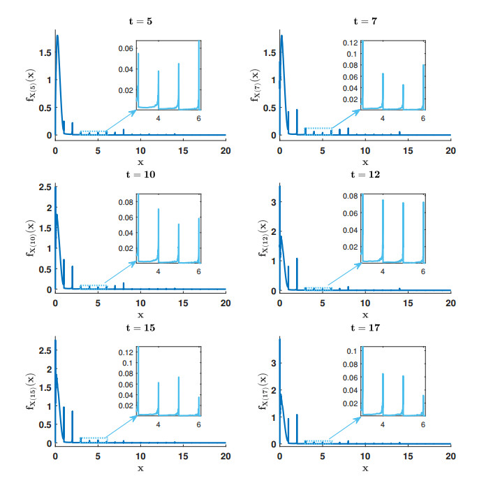
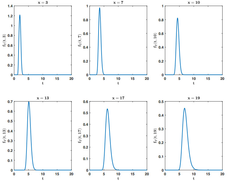
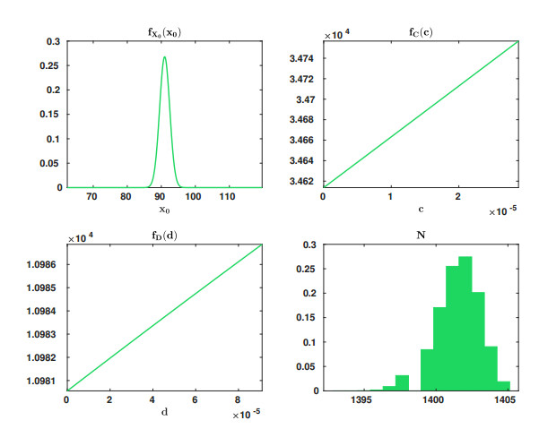
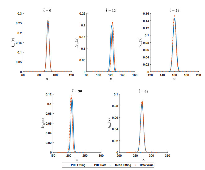
We provide a full stochastic description, via the first probability density function, of the solution of linear-quadratic logistic-type differential equation whose parameters involve both continuous and discrete random variables with arbitrary distributions. For the sake of generality, the initial condition is assumed to be a random variable too. We use the Dirac delta function to unify the treatment of hybrid (discrete-continuous) uncertainty. Under general hypotheses, we also compute the density of time until a certain value (usually representing the population) of the linear-quadratic logistic model is reached. The theoretical results are illustrated by means of several examples, including an application to modelling the number of users of Spotify using real data. We apply the Principle Maximum Entropy to assign plausible distributions to model parameters.
Citation: Clara Burgos, Juan Carlos Cortés, Elena López-Navarro, Rafael Jacinto Villanueva. Probabilistic analysis of linear-quadratic logistic-type models with hybrid uncertainties via probability density functions[J]. AIMS Mathematics, 2021, 6(5): 4938-4957. doi: 10.3934/math.2021290

Related Papers:

Abstract

We provide a full stochastic description, via the first probability density function, of the solution of linear-quadratic logistic-type differential equation whose parameters involve both continuous and discrete random variables with arbitrary distributions. For the sake of generality, the initial condition is assumed to be a random variable too. We use the Dirac delta function to unify the treatment of hybrid (discrete-continuous) uncertainty. Under general hypotheses, we also compute the density of time until a certain value (usually representing the population) of the linear-quadratic logistic model is reached. The theoretical results are illustrated by means of several examples, including an application to modelling the number of users of Spotify using real data. We apply the Principle Maximum Entropy to assign plausible distributions to model parameters.

References

[1]	R. Goebel, R. G. Sanfelice, A. R. Teel, Hybrid Dynamical Systems: Modeling, Stability, and Robustness, Princeton University Press, 2012.
[2]	J. Lunze, F. Lamnabhi-Lagarrigue, Handbook of Hybrid Systems Control: Theory, Tools, Applications, ser. Nonlinear Systems and Complexity, Cambridge University Press, 2009.
[3]	E. Villani, P. E. Miyagi, R. Valette, Modelling and Analysis of Hybrid Supervisory Systems: A Petri Net Approach, ser. Advances in Industrial Control, Springer, 2007.
[4]	X. Yang, X. Li, J. Lu, Z. Cheng, Synchronization of time-delayed complex networks with switching topology via hybrid actuator fault and impulsive effects control, IEEE Trans. Cybernetics, 50 (2019), 4043–4052.
[5]	H. Zhu, X. Li, J. Lu, Z. Cheng, Input-to-state stability of impulsive systems with hybrid delayed impulse effects, J. Appl. Anal. Comput., 50 (2019), 777–795.
[6]	X. Liu, P. Stechlinski, Infectious Disease Modeling: A Hybrid System Approach, ser. Nonlinear Systems and Complexity, Springer International Publishing, 19 (2017).
[7]	R. C. Smith, Uncertainly Quantification: Theory, Implementation, and Applications, ser. Computational Science & Engineering, SIAM, 2013.
[8]	E. Allen, Modeling with Itô Stochastic Differential Equations, Springer Science & Business Media, 22 (2007).
[9]	T. T. Soong, Random Differential Equations in Science and Engineering, New York: Academic Press, 1973.
[10]	F. B. Hanson, Applied Stochastic Processes and Control for Jump-Diffusions, SIAM, 2007.
[11]	J. Bertoin, Lévy processes, Cambridge University Press, 1996.
[12]	M. Grigoriu, Applied Non-Gaussian Processes, Prentice-Hall, 1995.
[13]	M. Grigoriu, Numerical solution of stochastic differential equations with Poisson and Lèvy white noise, Physical Rev. E, 80 (2009), 02670.
[14]	M. C. Casabán, J. C. Cortés, A. Navarro-Quiles, J. V. Romero, M. D. Roselló, R. J. Villanueva, A comprehensive probabilistic solution of random SIS-type epidemiological models using the random variable transformation technique, Commun. Nonlinear Sci. Numer. Simul., 32 (2016), 199–210. Available from: https://doi.org/10.1016/j.cnsns.2015.08.009.
[15]	F. A. Dorini, M. S. Cecconello, L. B. Dorini, On the logistic equation subject to uncertainties in the environmental carrying capacity and initial population density, Commun. Nonlinear Sci. Numer. Simul., 33 (2016), 160–173. Available from: https://doi.org/10.1016/j.cnsns.2015.09.009.
[16]	F. A. Dorini, M. C. C. Cunha, Statistical moments of the random linear transport equation, J. Comput. Phy., 227 (2008), 8541–8550. Available from: https://doi.org/10.1016/j.jcp.2008.06.002.
[17]	M. Hussein, M. Selim, A complete probabilistic solution for a stochastic milne problem of radiative transfer using KLE-RVT technique, J. Quantit. Spectrosc. Radiat. Transfer, 232 (2019), 54–65. doi: 10.1016/j.jqsrt.2019.04.034
[18]	J. C. Cortés, I. C. Lombana, R. J. Villanueva, Age-structured mathematical modeling approach to short-term diffusion of electronic commerce in spain, Math. Comput. Model., 52 (2010), 1045–1051, mathematical Models in Medicine, Business and Engineering 2009. Available from: http://www.sciencedirect.com/science/article/pii/S0895717710000944.
[19]	R. Cervelló-Royo, J. C. Cortés, A. Sánchez-Sánchez, F. J. Santonja, R. Shoucri, R. J. Villanueva, Probabilistic european country risk score forecasting using a diffusion model, In: Computational models of complex systems, Springer, (2014), 45–58.
[20]	J. Calatayud, J. C. Cortés, F. A. Dorini, M. Jornet, Solution of the finite Milne problem in stochastic media with RVT Technique, Comput. Appl. Math., 39 (2020), 288. doi: 10.1007/s40314-020-01343-z
[21]	R. F. Hoskins, Delta functions: Introduction to generalised functions, Horwood Publishing, 2009.
[22]	Matlab, Cupula Matlab, 2020, Available from: https://es.mathworks.com/help/stats/copularnd.html.
[23]	L. Devroye, Nonuniform random variate generation, Handbooks Oper. Res. Manage. Sci., 13 (2006), 83–121. doi: 10.1016/S0927-0507(06)13004-2
[24]	C. Burgos, J. C. Cortés, D. Martínez-Rodríguez, R. J. Villanueva, Modeling breast tumor growth by a randomized logistic model: A computational approach to treat uncertainties via probability densities, Europ. Phy. J. Plus, 135 (2020). Available from: https://doi.org/10.1140/epjp/s13360-020-00853-3.
[25]	J. V. Michalowicz, J. M. Nichols, F. Bucholtz, Handbook Differ. Entropy, CRC Press, 2013.
[26]	Statista, Number of Spotify monthly active users (maus) worldwide from 1st quarter 2015 to 3rd quarter 2020. Available from: https://www.statista.com/statistics/367739/spotify-global-mau/.
[27]	G. Casella, R. Berger, Statistical Inference, ser. Duxbury Advanced Series, New York: Brooks Cole, 2002.
[28]	The MathWorks Inc. (2020), Particle swarm optimization. Available from: https://es.mathworks.com/help/gads/particleswarm.html.

Reader Comments

Your name:*

Email:*
© 2021 the Author(s), licensee AIMS Press. This is an open access article distributed under the terms of the Creative Commons Attribution License (http://creativecommons.org/licenses/by/4.0)