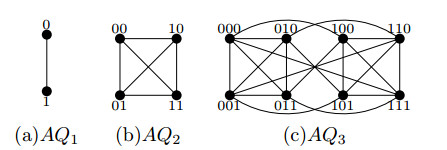
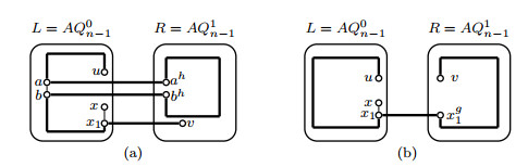
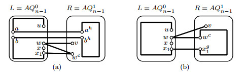
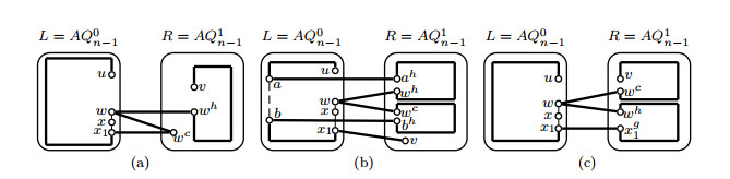
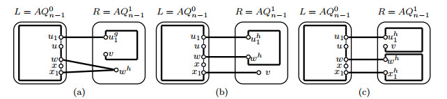
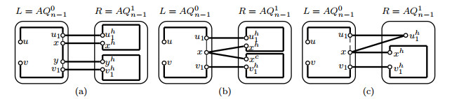
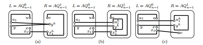
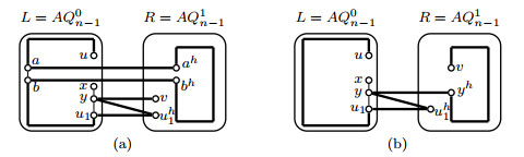
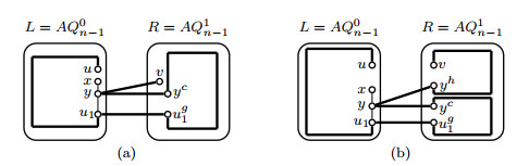
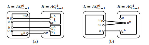
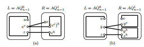
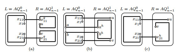
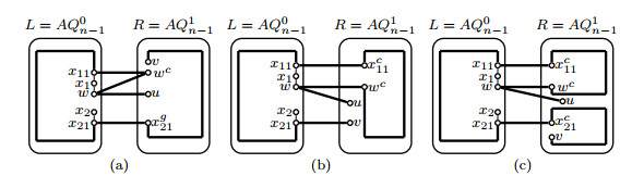
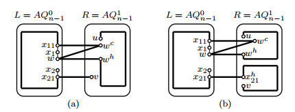
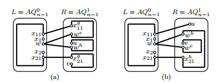
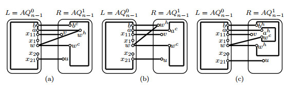
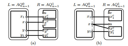
The augmented cube AQn is an outstanding variation of the hypercube Qn. It possesses many of the favorable properties of Qn as well as some embedded properties not found in Qn. This paper focuses on the fault-tolerant Hamiltonian connectivity of AQn. Under the assumption that F⊂V(AQn)∪E(AQn) with |F|≤2n−3, we proved that for any two different correct vertices u and v in AQn, there exists a fault-free Hamiltonian path that joins vertices u and v with the exception of (u,v), which is a weak vertex-pair in AQn−F(n≥4). It is worth noting that in this paper we also proved that if there is a weak vertex-pair in AQn−F, there is at most one pair. This paper improved the current result that AQn is 2n−4 fault-tolerant Hamiltonian connected. Our result is optimal and sharp under the condition of no restriction to each vertex.
Citation: Huifeng Zhang, Xirong Xu, Ziming Wang, Qiang Zhang, Yuansheng Yang. (2n−3)-fault-tolerant Hamiltonian connectivity of augmented cubes AQn[J]. AIMS Mathematics, 2021, 6(4): 3486-3511. doi: 10.3934/math.2021208
[1] | Yanling Wang, Shiying Wang . Edge-fault-tolerant strong Menger edge connectivity of bubble-sort graphs. AIMS Mathematics, 2021, 6(12): 13210-13221. doi: 10.3934/math.2021763 |
[2] | Huifen Ge, Shumin Zhang, Chengfu Ye, Rongxia Hao . The generalized 4-connectivity of folded Petersen cube networks. AIMS Mathematics, 2022, 7(8): 14718-14737. doi: 10.3934/math.2022809 |
[3] | Bo Zhu, Shumin Zhang, Jinyu Zou, Chengfu Ye . Structure connectivity and substructure connectivity of data center network. AIMS Mathematics, 2023, 8(4): 9877-9889. doi: 10.3934/math.2023499 |
[4] | Maryam Salem Alatawi, Ali Ahmad, Ali N. A. Koam, Sadia Husain, Muhammad Azeem . Computing vertex resolvability of benzenoid tripod structure. AIMS Mathematics, 2022, 7(4): 6971-6983. doi: 10.3934/math.2022387 |
[5] | Xiaogang Liu, Muhammad Ahsan, Zohaib Zahid, Shuili Ren . Fault-tolerant edge metric dimension of certain families of graphs. AIMS Mathematics, 2021, 6(2): 1140-1152. doi: 10.3934/math.2021069 |
[6] | Bo Zhu, Shumin Zhang, Huifen Ge, Chengfu Ye . The $ g $-extra $ H $-structure connectivity and $ g $-extra $ H $-substructure connectivity of hypercubes. AIMS Mathematics, 2023, 8(10): 24848-24861. doi: 10.3934/math.20231267 |
[7] | Zuo Wang, Hong Xue, Yingnan Pan, Hongjing Liang . Adaptive neural networks event-triggered fault-tolerant consensus control for a class of nonlinear multi-agent systems. AIMS Mathematics, 2020, 5(3): 2780-2800. doi: 10.3934/math.2020179 |
[8] | Xia Liu . A related problem on $ s $-Hamiltonian line graphs. AIMS Mathematics, 2022, 7(10): 19553-19561. doi: 10.3934/math.20221073 |
[9] | Weiwei Sun, Mengyang Qiu, Xinyu Lv . H∞ filter design for a class of delayed Hamiltonian systems with fading channel and sensor saturation. AIMS Mathematics, 2020, 5(4): 2909-2922. doi: 10.3934/math.2020188 |
[10] | Usman Babar, Haidar Ali, Shahid Hussain Arshad, Umber Sheikh . Multiplicative topological properties of graphs derived from honeycomb structure. AIMS Mathematics, 2020, 5(2): 1562-1587. doi: 10.3934/math.2020107 |
The augmented cube AQn is an outstanding variation of the hypercube Qn. It possesses many of the favorable properties of Qn as well as some embedded properties not found in Qn. This paper focuses on the fault-tolerant Hamiltonian connectivity of AQn. Under the assumption that F⊂V(AQn)∪E(AQn) with |F|≤2n−3, we proved that for any two different correct vertices u and v in AQn, there exists a fault-free Hamiltonian path that joins vertices u and v with the exception of (u,v), which is a weak vertex-pair in AQn−F(n≥4). It is worth noting that in this paper we also proved that if there is a weak vertex-pair in AQn−F, there is at most one pair. This paper improved the current result that AQn is 2n−4 fault-tolerant Hamiltonian connected. Our result is optimal and sharp under the condition of no restriction to each vertex.
Interconnection networks are of particular interest in the study of parallel computing systems. An interconnection network can be modeled as a graph G=(V,E), where V expresses the vertex set and E expresses the edge set. Exploring the structures of G is essential for designing a suitable topology for such an interconnection network. Topology structure has a crucial impact on the overall performance of the network. It determines the physical distribution of network nodes/links and the connection relationship between them. It also determines the number of hops in message transmission and the length of links per hop. Therefore, the topology has a great influence on the delay and power consumption. In addition, because the topology determines the number of available transmission paths between nodes, it also affects the distribution of network traffic, network bandwidth and transmission performance.
The hypercube Qn is one of the most prevalent interconnection networks among all the popular parallel network topologies that possess properties such as logarithmic diameter, high symmetry, linear bisection width. The n-dimensional augmented cube AQn is an outstanding variation of the hypercube Qn. It possesses many of the favorable properties of Qn as well as some embedded properties not found in Qn. Much research has been conducted on this type of augmented cube, and it appears frequently in the literatures [1,3,4,12,13,14,16,20,22].
In the last several years, the path embedding problem has become one of the most-studied graph embedding problems, appearing prolifically in the literatures[5,6,10,14]. The fault-tolerant path embedding problem has also been the subject of frequent investigation, as is evident in the literatures [3,4,7,11,10,22,23,24].
A path (or cycle) is considered a Hamiltonian path (or Hamiltonian cycle) if it passes through every vertex of graph G once and only once. A graph is said to be Hamiltonian if it contains at least one Hamiltonian cycle. One of the most challenging contemporary problems in graph theory is identifying a necessary and sufficient condition for a graph to be considered Hamiltonian. A graph G is regarded as Hamiltonian connected if for any pair of distinct vertices u and v, a Hamiltonian path Puv exists. Hamiltonian paths and cycles have applicability for practical problems such as online optimization of complex, flexible manufacturing systems [25], wormhole routing [26], deadlock-free routing and broadcasting algorithms [27]. Applicability for such problems have been a driving force for the study of networks embedded with Hamiltonian paths.
In large interconnection networks, vertices(or edges) show a propensity for faultiness. This faultiness demands attention, as fault-tolerance serves as an important index of a network's stability. A graph G can be said to be k-fault-tolerant Hamiltonian connected if G−F remains Hamiltonian connected for any F⊂V(G)∪E(G) with |F|≤k.
Hsu et al.[3] proved that AQn(n≥1) is Hamiltonian-connected. They also showed that AQn is (2n−3)-fault-tolerant Hamiltonian and (2n−4)-fault-tolerant Hamiltonian connected for n≥4 even when faulty elements occur. Soon after, Wang et al.[4] proved that AQn is (2n−5)-fault-tolerant Panconnected for n≥3. We improved this result and showed that if F⊂V(AQn)∪E(AQn) with |F|≤2n−4, then for any two distinct error-free vertices u and v with distance d, there exists an error-free path Puv of length l with max{d+2,4}⩽l⩽2n−fv−1 in AQn−F(n≥4)[22].
In this paper, we show that for any two distinct error-free vertices u and v, there exists a fault-free Hamiltonian path Puv that joins vertices u and v with the exception of (u,v), which is a weak vertex-pair in AQn−F(n≥4) under the assumption that F⊂V(AQn)∪E(AQn) with |F|≤2n−3.
The rest of this paper is outlined as follows. Section 2 introduces the definitions and properties of the augmented cubes AQn. In Section 3, we investigate some lemmas of AQn to be used in our proofs. Section 4 proves the main theorem. Finally, Section 5 concludes the paper.
In this section, we will introduce the definition of AQn and basic properties used in this paper.
Definition 2.1. The n-dimensional augmented cube AQn, proposed by Choudum and Sunitha[16], can be defined recursively as follows.
AQ1 is a complete graph K2 with vertex set {0,1}. For n≥2, AQn is obtained by taking two copies of the augmented cube AQn−1 denoted by 0AQn−1 and 1AQn−1, and adding 2×2n−1 edges between the two copies as follows.
Let V(0AQn−1)={0xn−1…x2x1|xi∈{0,1}} and V(1AQn−1)={1xn−1…x2x1|xi∈{0,1}}. A vertex x∈V(0AQn−1) is adjacent to a vertex y∈V(1AQn−1) if and only if either:
(1) xi=yi for 1≤i≤n−1; in this case, xy is called a hypercube edge and we set x=yhn or y=xhn, or
(2) xi=¯yi for 1≤i≤n−1; in this case, xy is called a complement edge and we set x=ycn or y=xcn.
And an edge between x=xnxn−1…xi…x2x1 and y=xnxn−1…¯xi…x2x1(xi∈{0,1}, 2≤i≤n) is called an i-dimensional hypercube edge, setting x=yhi or y=xhi, an edge between x=xnxn−1…xi…x2x1 and y=xnxn−1…¯xi…¯x2x1(xi∈{0,1}, 1≤i≤n) is called an i-dimensional complement edge, setting x=yci or y=xci. For any vertex u in AQn, we use uh to denote uhn and use uc to denote ucn. Examples of the augmented cubes AQ1, AQ2 and AQ3 are shown in Figure 1(a)–(c), respectively.
AQn is (2n−1)-regular that has, naturally, 2n vertices. For the sake of simplicity, we write this as L=0AQn−1 and R=1AQn−1. Let NAQn(x) express the set of vertices which are incident to vertex x and EAQn(x) express the set of edges which are incident to vertex x. For each vertex x∈V(L)(or V(R)), let NL(x)(or NR(x)) express the set of vertices adjacent to x in V(L)(or V(R)), EC signify the set of edges joining L to R and EL(x)(or ER(x)) serve as the set of edges which are incident to vertex x in L(or R).
For two distinct vertices u and v in G, a path Puv from vertex u to vertex v of length k is a sequence of different vertices (x0,x1,…,xk), where x0=u, xk=v, xi−1xi∈E(G) for each i=1,2,…,k, and k is the number of edges in Puv, called the length of Puv. The distance between vertices u and v, denoted by duv, is the length of a shortest path from vertex u to vertex v in G.
Let Puv=(u,u1,u2,⋯,uk−1,v) be a path from vertex u to vertex v. A subsequence (ui,ui+1,⋯,uj) of Puv is called a subpath of Puv, denoted by Puv(ui,uj). We can write Puv=(u,u1,⋯,ui,Puv(ui,uj),uj,⋯uk−1,v). A cycle is a path Puv with u=v. We use C=(u,u1,u2,⋯,uk−1,u) to denote a cycle containing vertex u.
We first give the useful definitions and properties about AQn as follows.
Proposition 2.1. Let uv be an edge in AQn(n≥2) [4]. If uv is not an (n−1)-dimensional complement edge, then uh, uc, vh and vc are all distinct. Otherwise, uh=vc, uc=vh.
Proposition 2.2. For any two distinct vertices u and v of AQn, we have |(NAQn(u)∪EAQn(u))∩(NAQn(v)∪EAQn(v))|≤5.
Proof. Let m be the adjacent vertex of vertex u. Then
m={ucj=unun−1⋯uj+1ˉujˉuj−1⋯ˉu2ˉu1,1≤j≤n.uhj=unun−1⋯uj+1ˉujuj−1⋯u2u1,2≤j≤n. |
If there exists at least one common adjacent vertex between any two distinct vertices u and v of AQn, then duv≤2. We divided to the following two cases to prove.
Case 1. duv=1.
Case 1.1. v=uci(1≤i≤n). Then v=unun−1⋯ui+1ˉuiˉui−1⋯ˉu2ˉu1.
m∈N(v) if and only if
m={uci+1=unun−1⋯ˉui+1ˉuiˉui−1⋯ˉu2ˉu1,1≤i≤n−1.uci−1=unun−1⋯ui+1uiˉui−1⋯ˉu2ˉu1,2≤i≤n.uhi=unun−1⋯ui+1ˉuiui−1⋯u2u1,2≤i≤n.uhi+1=unun−1⋯ˉui+1uiui−1⋯u2u1,1≤i≤n−1. |
Then NAQn(u)∩NAQn(v)={uci+1,uci−1,uhi,uhi+1} for 2≤i≤n−1, NAQn(u)∩NAQn(v)={uci+1,uhi+1} for i=1, NAQn(u)∩NAQn(v)={uci−1,uhi} for i=n.
Case 1.2. v=uhi(2≤i≤n). Then v=unun−1⋯ui+1ˉuiui−1⋯u2u1.
m∈N(v) if and only if
m={uci−1=unun−1⋯ui+1uiˉui−1⋯ˉu2ˉu1,2≤i≤n.uci=unun−1⋯ui+1ˉuiˉui−1⋯ˉu2ˉu1,2≤i≤n. |
Then NAQn(u)∩NAQn(v)={uci−1,uci} for 2≤i≤n.
Case 2. duv=2.
Case 2.1. v=ucick(1≤i<k≤n, k≠i+1). Then v=unun−1⋯uk+1ˉukˉuk−1⋯ˉui+1uiui−1⋯u2u1. m∈N(v) if and only if
m={uci=unun−1⋯uk+1ukuk−1⋯ui+1ˉuiˉui−1⋯ˉu2ˉu1,uck=unun−1⋯uk+1ˉukˉuk−1⋯ˉui+1ˉuiˉui−1⋯ˉu2ˉu1,uhk=unun−1⋯uk+1ˉukui+1uiui−1⋯u2u1,k=i+2.uhi+1=unun−1⋯uk+1ukˉui+1uiui−1⋯u2u1,k=i+2. |
Then NAQn(u)∩NAQn(v)={uci,uck,uhk,uhi+1} for k=i+2 and NAQn(u)∩NAQn(v)={uci,uck} for k≠i+2.
Case 2.2. v=ucihk(1≤i<k≤n, k≠i+1). Then v=unun−1⋯uk+1ˉukuk−1⋯ui+1ˉuiˉui−1⋯ˉu2ˉu1. m∈N(v) if and only if
m={uci=unun−1⋯uk+1ukuk−1⋯ui+1ˉuiˉui−1⋯ˉu2ˉu1,uhk=unun−1⋯uk+1ˉukuk−1⋯ui+1uiui−1⋯u2u1,uck=unun−1⋯uk+1ˉukˉui+1ˉuiˉui−1⋯ˉu2ˉu1,k=i+2.uhi+1=unun−1⋯uk+1ukˉui+1uiui−1⋯u2u1,k=i+2. |
Then NAQn(u)∩NAQn(v)={uci,uhk,uck,uhi+1} for k=i+2 and NAQn(u)∩NAQn(v)={uci,uhk} for k≠i+2.
Case 2.3. v=uhihk(2≤i<k≤n). Then v=unun−1⋯uk+1ˉukuk−1⋯ui+1ˉuiui−1⋯u2u1. m∈N(v) if and only if
m={uhi=unun−1⋯uk+1ukuk−1⋯ui+1ˉuiui−1⋯u2u1,uhk=unun−1⋯uk+1ˉukuk−1⋯ui+1uiui−1⋯u2u1,uci−1=unun−1⋯uk+1ukuiˉui−1⋯ˉu2ˉu1,k=i+1.uck=unun−1⋯uk+1ˉukˉuiˉui−1⋯ˉu2ˉu1,k=i+1. |
Then NAQn(u)∩NAQn(v)={uhi,uhk,uci−1,uck} for k=i+1 and NAQn(u)∩NAQn(v)={uhi,uhk} for k≠i+1.
Case 2.4. v=uhick(2≤i<k≤n). Then v=unun−1⋯uk+1ˉukˉuk−1⋯ˉui+1uiˉui−1⋯ˉu2ˉu1. m∈N(v) if and only if
m={uhi=unun−1⋯uk+1ukuk−1⋯ui+1ˉuiui−1⋯u2u1,uck=unun−1⋯uk+1ˉukˉuk−1⋯ˉui+1ˉuiˉui−1⋯ˉu2ˉu1,uci−1=unun−1⋯uk+1ukuiˉui−1⋯ˉu2ˉu1,k=i+1.uhk=unun−1⋯uk+1ˉukuiui−1⋯u2u1,k=i+1. |
Then NAQn(u)∩NAQn(v)={uhi,uck,uci−1,uhk} for k=i+1 and NAQn(u)∩NAQn(v)={uhi,uck} for k≠i+1.
Combining the above cases, we have that |NAQn(u)∩NAQn(v)|≤4. If uv∈E(AQn), then |(NAQn(u)∪EAQn(u))∩(NAQn(v)∪EAQn(v))|≤5. If uv∉E(AQn), then |(NAQn(u)∪EAQn(u))∩(NAQn(v)∪EAQn(v))|≤4. Hence, we have |(NAQn(u)∪EAQn(u))∩(NAQn(v)∪EAQn(v))|≤5.
Definition 2.2. Let F⊂V(AQn)∪E(AQn) with |F|=2n−3. If AQn−F include a vertex w with NAQn−F(w)={w1,w2}, then w is considered a weak 2-degree vertex and (w1,w2) is considered a w-weak vertex pair(or a weak vertex pair, for short).
Take F={a,b} for an example, we know that w is a weak 2-degree vertex and (w1,w2) is a weak vertex-pair in AQ3−F(See Figure 2).
Because it is impossible for any error-free path Pw1w2 of length l with l≥3 to contain the weak 2-degree vertex w, no error-free Hamiltonian path that joins vertices w1 and w2 exists in AQn−F. Fortunately, at most one weak 2-degree vertex w and at most one w-weak vertex-pair exist in AQn−F(n≥5) for any F⊂V(AQn)∪E(AQn) with |F|=2n−3. We shall provide proof of this fact in Proposition 2.3.
Definition 2.3. If (w1,w2) is not a weak vertex-pair for arbitrary vertex w∈V(AQn−F), then (w1,w2) is called a normal vertex pair.
Proposition 2.3. Let F⊂V(AQn)∪E(AQn) with |F|≤2n−1(n≥6). Then there exists at most one vertex z∈V(AQn−F) such that dAQn−F(z)≤2.
Proof. Assume that there exist two vertices z1,z2 such that dAQn−F(z1)≤2 and dAQn−F(z2)≤2. Since AQn is a (2n−1)-regular graph, we have |F∩(NAQn(z1)∪EAQn(z1))|≥2n−3 and |F∩(NAQn(z2)∪EAQn(z2))|≥2n−3.
By Proposition 2.2, |(NAQn(z1)∪EAQn(z1))∩(NAQn(z2)∪EAQn(z2))|≤5. Then |F∩(NAQn(z1)∪EAQn(z1))|+|F∩(NAQn(z2)∪EAQn(z2))|-|F∩(NAQn(z1)∪EAQn(z1))∩(NAQn(z2)∪EAQn(z2))|≥2(2n−3)−5=4n−11>2n−1(n≥6), a contradiction to |F|≤2n−1.
Hence, at most one vertex z∈V(AQn−F) exists in AQn−F such that dAQn−F(z)≤2 for any F⊂V(AQn)∪E(AQn) with |F|≤2n−1. By Proposition 2.3, we can obtain the Corollary 2.1 as follows.
Corollary 2.1. Let F⊂V(AQn)∪E(AQn) with |F|≤2n−3. Then at most a weak 2-degree vertex w and at most a w-weak vertex-pair exist in AQn−F(n≥6).
Denote FL=F∩L, FR=F∩R, FC=F∩EC, Fv=F∩V(AQn), Fe=F∩E(AQn), FLv=V(L)∩FL, FRv=V(R)∩FR, fv=|Fv|, fLv=|FLv|, fRv=|FRv|.
We need the following lemmas.
Lemma 3.1. AQn(n≥3) is (2n−4)-fault-tolerant Hamiltonian connected and (2n−3)-fault-tolerant Hamiltonian [3].
Lemma 3.2. If |FL|=2n−3(n≥6), then for arbitrary vertex-pair (u,v) with u,v∈V(L), there exist two faulty elements x1,x2∈FL such that (u,v) is a normal vertex-pair in L−(FL−{x1,x2}).
Proof. We use the following two cases to prove.
Case 1. (u,v) is a w-weak vertex pair in L−FL. Then dL−FL(w)=2 and |FL∩(NL(w)∪EL(w))|=2n−5. By Proposition 2.3, w is the unique vertex in L−FL with dL−FL(w)≤2.
So, we can choose two elements x1,x2∈FL∩(NL(w)∪EL(w)). Let FL1=FL−{x1,x2}, then dL−FL1(w)=4. Hence, (u,v) is a normal vertex pair in L−FL1.
Case 2. (u,v) is a normal vertex pair in L−FL. Let vertex z∈L−FL with the least degree.
Case 2.1. δ(L−FL)=0, then FL⊂NL(z)∪EL(z), dL−FL(z)=0.
Case 2.1.1. z∈{u,v}. Assume that u=z(When v=z, the same proofs apply).
By Proposition 2.3, u is the unique vertex in L−FL with dL−FL(u)≤2. Then (u,v) is a normal vertex-pair in L−(FL−{x1,x2}) for arbitrary two elements x1,x2 of FL.
Case 2.1.2. z∉{u,v}.
By Proposition 2.3, z is the unique vertex in L−FL with dL−FL(z)≤2. There exist two elements x1,x2∈FL∩(NL(z)∪EL(z)) with x1,x2∉{uz,vz}. Let FL1=FL−{x1,x2}, then dL−FL1(z)=2 and NL−FL1(z)≠{u,v}. Hence, (u,v) is a normal vertex pair in L−FL1.
Case 2.2. δ(L−FL)=1. Then |FL∩(NL(z)∪EL(z))|=2n−4 and dL−FL(z)=1.
By Proposition 2.3, z is the unique vertex in L−FL with dL−FL(z)≤2. There exist two elements x1,x2∈FL∩(NL(z)∪EL(z)). Let FL1=FL−{x1,x2}, then dL−FL1(z)=3. Then (u,v) is a normal vertex pair in L−FL1.
Case 2.3. δ(L−FL)≥2.
Then (u,v) is a normal vertex-pair in L−(FL−{x1,x2}) for arbitrary two elements x1,x2 of FL.
The Lemma holds.
By a similar argument to Lemma 3.2, we can get the following Lemma.
Lemma 3.3. If |FL|=2n−4(n≥6), then for arbitrary vertex-pair (u,v) with u,v∈V(L), there is a faulty element x∈FL such that (u,v) is a normal vertex-pair in L−(FL−{x}).
Lemma 3.4. Let F⊂V(AQn)∪E(AQn) with |F|≤2 and x,y,z,w be four distinct vertices in AQn(n≥4). Then two disjoint paths Pxy, Pzw such that V(Pxy)∪V(Pzw)=V(AQn−F) will exist.
Proof. We prove the lemma by induction on n≥4. The induction basis for n=4 holds by computer program. Suppose that the lemma holds for n−1 with n≥5, then we must show the lemma holds for n.
Case 1. x,y,z,w∈V(L).
By induction hypothesis, two disjoint paths Pxy, Pzw with V(Pxy)∪V(Pzw)=V(L−FL) exist in L−FL. Assume that |V(Pxy)|≥|V(Pzw)|. Then |V(Pxy)|2≥⌈2n−22⌉/2≥7(n≥5). Since |F|≤2, we can choose an edge x1y1⊂E(Pxy) such that xh1,yh1,x1xh1,y1yh1∉F. By Lemma 3.1, a Hamiltonian path Pxh1yh1 will exist in R−FR. Let P1xy=(x,Pxy(x,x1),x1,xh1,Pxh1yh1,yh1,y1,Pxy(y1,y),y). Then P1xy,Pzw are two desired paths in AQn−F(see Figure 3(a)).
Case 2. x,y,z∈V(L), w∈V(R).
Since |EC|−12=2n−12≥20(n≥5), an error-free edge z1zh1 can be chosen form EC such that z1∉{x,y,z}, zh1≠w and z1,zh1∉F. By induction hypothesis, two disjoint paths Pxy, Pzz1 with V(Pxy)∪V(Pzz1)=V(L−FL) exist in L−FL. By Lemma 3.1, we can find a Hamiltonian path Pzh1w in R−FR. Let Pzw=(z,Pzz1,z1,zh1,Pzh1w,w). Then Pxy,Pzw are two desired paths in AQn−F(see Figure 3(b)).
Case 3. x,y∈V(L), z,w∈V(R).
By Lemma 3.1, we can find a Hamiltonian path Pxy in L−FL and a Hamiltonian path Pzw in R−FR. Then Pxy,Pzw are two desired paths in AQn−F(see Figure 4(a)).
Case 4. x,z∈V(L), y,w∈V(R).
Since |EC|−12=2n−12≥20(n≥5), there are two error-free disjoint edges x1xh1,z1zh1 such that x1,z1∉{x,z}, xh1,zh1∉{y,w} and x1,xh1,z1,zh1∉F. By induction hypothesis, two disjoint paths Pxx1, Pzz1 with V(Pxx1)∪V(Pzz1)=V(L−FL) exist in L−FL and two disjoint paths Pxh1y, Pzh1w with V(Pxh1y)∪V(Pzh1w)=V(R−FR) exist in R−FR. Let Pxy=(x,Pxx1,x1,xh1,Pxh1y,y), Pzw=(z,Pzz1,z1,zh1,Pzh1w,w). Then Pxy,Pzw are two desired paths in AQn−F(see Figure 4(b)).
The lemma holds.
Lemma 3.5. Let x,y,z,w,a,b be six distinct vertices in AQn(n≥4). Then there exist three disjoint paths Pxy, Pzw, and Pab such that V(Pxy)∪V(Pzw)∪V(Pab)=V(AQn).
Proof. We prove the lemma by induction on n≥4. The induction basis for n=4 holds by computer program. Suppose the lemma holds for n−1 with n≥5, then we must show the lemma holds for n.
Case 1. x,y,z,w,a,b∈V(L).
By induction hypothesis, three disjoint paths Pxy, Pzw and Pab with V(Pxy)∪V(Pzw)∪V(Pab)=V(L) will exist in L. Let x1y1∈E(Pxy). By Lemma 3.1, a Hamiltonian path Pxh1yh1 can be found in R. Let P1xy=(x,Pxy(x,x1),x1,xh1,Pxh1yh1,yh1,y1,Pxy(y1,y),y). Then P1xy,Pzw,Pab are three desired paths in AQn(see Figure 5(a)).
Case 2. x,y,z,w,a∈V(L), b∈V(R).
Choose a vertex a1 from V(L)−{x,y,z,w,a} such that there exists a vertex ag1∈{ah1,ac1} with ag1≠b. By induction hypothesis, three disjoint paths Pxy, Pzw and Paa1 with V(Pxy)∪V(Pzw)∪V(Paa1)=V(L) will exist in L. By Lemma 3.1, a Hamiltonian path Pag1b can be found in R. Let Pab=(a,Paa1,a1,ag1,Pag1b,b). Then Pxy,Pzw,Pab are three desired paths in AQn(see Figure 5(b)).
Case 3. x,y,z,w∈V(L), a,b∈V(R).
By Lemma 3.4, two disjoint paths Pxy, Pzw with V(Pxy)∪V(Pzw)=V(L) exist in L. By Lemma 3.1, we can find a Hamiltonian path Pab in R. Then Pxy,Pzw,Pab are three desired paths in AQn(see Figure 5(c)).
Case 4. x,y,z,a∈V(L), w,b∈V(R).
Since |EC|−12=2n−12≥20, there are two disjoint edges z1zh1,a1ah1 such that z1,a1∉{x,y,z,a} and zh1,ah1∉{w,b}. By induction hypothesis, three disjoint paths Pxy, Pzz1 and Paa1 with V(Pxy)∪V(Pzz1)∪V(Paa1)=V(L) will exist in L. And by Lemma 3.4, two disjoint paths Pzh1w, Pah1b with V(Pzh1w)∪V(Pah1b)=V(R) will exist in R. Let Pzw=(z,Pzz1,z1,zh1,Pzh1w,w) and Pab=(a,Paa1,a1,ah1,Pah1b,b). Then Pxy,Pzw,Pab are three desired paths in AQn(see Figure 6(a)).
Case 5. x,z,a∈V(L), y,w,b∈V(R).
Since |EC|−12=2n−12≥20, there are three disjoint edges x1xh1,z1zh1,a1ah1 such that x1,z1,a1∉{x,z,a} and xh1,zh1,ah1∉{y,w,b}. By induction hypothesis, three disjoint paths Pxx1, Pzz1 and Paa1 with V(Pxx1)∪V(Pzz1)∪V(Paa1)=V(L) will exist in L and three disjoint paths Pxh1y, Pzh1w, Pah1b with V(Pxh1y)∪V(Pzh1w)∪V(Pah1b)=V(R) will exist in R. Let Pxy=(x,Pxx1,x1,xh1,Pxh1y,y), Pzw=(z,Pzz1,z1,zh1,Pzh1w,w) and Pab=(a,Paa1,a1,ah1,Pah1b,b). Then Pxy,Pzw,Pab are three desired paths in AQn(see Figure 6(b)).
Case 6. x,y,a∈V(L), z,w,b∈V(R).
Since |EC|−12=2n−12≥20, there is an edge a1ah1 such that a1∉{x,y,a} and ah1∉{z,w,b}. By Lemma 3.4, two disjoint paths Pxy and Paa1 with V(Pxy)∪V(Paa1)=V(L) will exist in L and two disjoint paths Pzw and Pah1b with V(Pzw)∪V(Pah1b)=V(R) will exist in R. Let Pab=(a,Paa1,a1,ah1,Pah1b,b). Then Pxy,Pzw,Pab are three desired paths in AQn(see Figure 6(c)).
The lemma holds.
Theorem 4.1. Let F⊂V(AQn)∪E(AQn) with |F|≤2n−3(n≥4). Then for arbitrary two different vertices u and v in AQn−F, there exists an error-free Hamiltonian path Puv except (u,v) is a weak vertex-pair in AQn−F.
Proof. For |F|≤2n−4, the theorem holds by Lemma 3.1. We only need to consider |F|=2n−3.
Now, we prove the theorem by induction on n≥4. The induction basis for n=4,5 holds by computer program (https://github.com/ZhangHeidi/Hypercubes/blob/master/vcn02.c). Supposing that the theorem holds for n−1 with n≥6, we must show the theorem holds for n.
We may assume |FR|≤|FL|(When |FR|≥|FL|, the same proofs apply). Then |FR|≤⌊2n−32⌋≤n−1. Notice that |NR(x)|=2n−3 for any vertex x∈R, we have |NR−FR(x)|≥n−2≥4. Thus R−FR does not contain weak vertex-pairs.
Case 1. |FL|≤2n−5.
Case 1.1. u,v∈V(L−FL) or u,v∈V(R−FR). Suppose that u,v∈V(L−FL).
Case 1.1.1. (u,v) is a w-weak vertex-pair in L−FL, i.e., NL−FL(w)={u,v}. Since |NL(w)|=2n−3, we have |FL|=2n−5 and |FR|+|FC|=2. Note that (u,v) is a normal vertex-pair in AQn−F, we can choose a vertex wg from {wh,wc} such that wg,wwg∉F.
Because |V(L)−FL−{u,w,v}|≥2n−1−(2n−5)−3≥22(n≥6) and |FR|+|FC|=2, there is a vertex y∈V(L)−FL−{u,w,v} such that yh,yyh∉F and yh≠wg. By Corollary 2.1, (u,y) is a normal vertex-pair in L−FL. By induction hypothesis, a Hamiltonian path Puy exists in L−FL. Notice that NL−FL(w)={u,v}, then NPuy(w)={u,v}. Since |FR|≤2≤2n−6, by Lemma 3.1, a Hamiltonian path Pwgyh exists in R−FR. An error-free Hamiltonian path Puv=(u,w,wg,Pwgyh,yh,y,Puy(y,v),v) can therefore be found(see Figure 7(a)).
Case 1.1.2. (u,v) is a normal vertex-pair in L−FL.
Since |FL|≤2n−5, by induction hypothesis, a Hamiltonian path Puv exists in L−FL. By ⌊luv+12⌋−(2n−3)=⌊2n−1−fLv2⌋−(2n−3)≥3, we can choose an edge ab∈E(Puv) such that ah,bh,aah,bbh∉F. By induction hypothesis, a Hamiltonian path Pahbh exists in R−FR. An error-free Hamiltonian path P1uv=(u,Puv(u,a),a,ah,Pahbh,bh,b,Puv(b,v),v) can therefore be found(see Figure 7(b)).
Case 1.2. u∈V(L−FL) and v∈V(R−FR).
According to the definition of AQn, |EC|=2n. Since |EC|−2|F|=2n−2(2n−3)≥46(n≥6), there is an error-free edge ab∈EC such that a,b∉{u,v}, a,b∉F and (u,a) is a normal vertex-pair in L−FL. By induction hypothesis, a Hamiltonian path Pua in L−FL and a Hamiltonian path Pbv in R−FR exist. An error-free Hamiltonian path Puv=(u,Pua,a,b,Pbv,v) can therefore be found(see Figure 7(c)).
Case 2. |FL|=2n−4. Then |FR|+|FC|=1.
Case 2.1. u,v∈V(L−FL).
By Lemma 3.3, we can choose an element f∈FL such that (u,v) is a normal vertex-pair in L−(FL−{f}). Let FL1=FL−{f}. Then |FL1|=2n−5. By induction hypothesis, a Hamiltonian path Puv exists in L−FL1.
Case 2.1.1. f∈V(Puv)∪E(Puv).
If f∈E(L)∩FL, say f=ab; if f∈V(L)∩FL, say NPuv(f)={a,b}; let Puv=(u,Puv(u,a),a,f,b,Puv(b,v),v). Suppose that |{ah,bh,aah,bbh}∩F|≤|{ac,bc,aac,bbc}∩F|.
Case 2.1.1.1. |{ah,bh,aah,bbh}∩F|=0.
Since |FR|≤1≤2n−6, by Lemma 3.1, a Hamiltonian path Pahbh exists in R−FR. An error-free Hamiltonian path P1uv=(u,Puv(u,a),a,ah,Pahbh,bh,b,Puv(b,v),v) can therefore be found(see Figure 8(a)).
Case 2.1.1.2. |{ah,bh,aah,bbh}∩F|=1. Then |{ac,bc,aac,bbc}∩F|=1.
Notice that |FR|+|FC|=1, we have {ah,bh,aah,bbh}∩F={ac,bc,aac,bbc}∩F, i.e., {ah,bh,aah,bbh}={ac,bc,aac,bbc}. Then by Proposition 2.1, a=bcn−1, ah=bc and ac=bh. Suppose that ah∈F, then bh∉F. Let a1b1∈E(Puv) with a1,b1∉{a,b} and FR1=FR+{bh}. Then |FR1|≤2≤2n−6. By Lemma 3.1, a Hamiltonian path Pah1bh1 exists in R−FR1. An error-free Hamiltonian path P1uv=(u,Puv(u,a),a,bh,b,Puv(b,a1),a1,ah1,Pah1bh1,bh1,b1,Puv(b1,v),v) can therefore be found(see Figure 8(b)).
Case 2.1.2. f∉V(Puv)∪E(Puv).
Then an edge a2b2 can be chosen from Puv with ah2,bh2,a2ah2,b2bh2∉F. Since |FR|≤1≤2n−6. By Lemma 3.1, a Hamiltonian path Pah2bh2 exists in R−FR. An error-free Hamiltonian path P1uv=(u,Puv(u,a2),a2,ah2,Pah2bh2,bh2,b2,Puv(b2,v),v) can therefore be found(see Figure 8(c)).
Case 2.2. u∈V(L−FL) and v∈V(R−FR).
Case 2.2.1. |FLv|≥1. There is a vertex x∈FLv. Let FL1=FL−{x}, then |FL1|=|FL|−1=2n−5.
Case 2.2.1.1. (u, x) is a normal vertex-pair in L-F^L_1 .
By induction hypothesis, a Hamiltonian path P_{ux} exists in L-F^L_1 . Let N_{P_{ux}}(x) = x_1 . Since |F^R|+|F^C| = 1 , there is a vertex x_1^g\in \{x_1^h, x_1^c\} such that x_1^g, x_1x_1^g\notin F .
(1) x_1^g = v . Choose an edge ab\in E(P_{ux}) such that a^h, b^h, aa^h, bb^h\notin F and a, b\notin \{x, x_1\} . Let F_1^R = F^R+\{v\} . Then |F_1^R|\leq2\leq 2n-6 . By Lemma 3.1, a Hamiltonian path P_{a^hb^h} exists in R-F_1^R . An error-free Hamiltonian P_{uv} = (u, P_{ux}(u, a), a, a^h, P_{a^hb^h}, b^h, b, P_{ux}(b, x_1), x_1, v) can therefore be found(see Figure 9(a)).
(2) x_1^g\neq v . Since |F^R|\leq1\leq 2n-6 . By Lemma 3.1, a Hamiltonian path P_{x_1^gv} exists in R-F^R . An error-free Hamiltonian path P_{uv} = (u, P_{ux}(u, x_1), x_1, x_1^g, P_{x_1^gv}, v) can therefore be found(see Figure 9(b)).
Case 2.2.1.2. (u, x) is a w -weak vertex-pair in L-F^L_1 . Then N_{L-F^L_1}(w) = \{u, x\} , i.e., N_{L-F^L}(w) = u .
By Corollary 2.1., (u, w) is a normal vertex-pair in L-F^L_1 . Since |F^L_1| = 2n-5 , by induction hypothesis, a Hamiltonian path P_{uw} exists in L-F^L_1 . By N_{L-F^L_1}(w) = \{u, x\} , we have N_{P_{uw}}(w) = \{x\} . Let N_{P_{uw}}(x) = \{x_1\} with x_1\neq w .
(1) |\{w^h, w^c\}\cap F| = 0 .
(1.1) v\in \{w^h, w^c\} , assume that v = w^h . If x_1 = w^{c_{n-1}} , then by Proposition 2.1, x_1^h = w^c, x_1^c = w^h . We can choose an edge ab\in E(P_{uw}) such that a^h, b^h, aa^h, bb^h\notin F and a, b\notin \{w, x, x_1\} , then v, w^c\notin \{a^h, b^h\} . Let F^R_1 = F^R+\{v, w^c\} . Then |F^R_1|\leq3\leq 2n-6 . By Lemma 3.1, a Hamiltonian path P_{a^hb^h} exists in R-F_1^R . An error-free Hamiltonian path P_{uv} = (u, P_{uw}(u, a), a, a^h, P_{a^hb^h}, b^h, b, P_{uw}(b, x_1), x_1, w^c, w, v) can therefore be found(see Figure 10(a)). If x_1\neq w^{c_{n-1}} , then by Proposition 2.1, x_1^h\neq w^c, x_1^c\neq w^h . There exists an error-free vertex x^g_1\in\{x^c_1, x^h_1\} such that x^g_1, x_1x^g_1\notin F . We have x^g_1\notin \{w^c, v\} . Let F_1^R = F^R+\{v\} . Then |F_1^R|\leq2\leq2n-6 . By Lemma 3.1, a Hamiltonian path P_{x^g_1w^c} exists in R-F_1^R . An error-free Hamiltonian path P_{uv} = (u, P_{uw}(u, x_1), x_1, x_1^g, P_{x^g_1w^c}, w^c, w, v) can therefore be found(see Figure 10(b)).
(1.2) v\notin \{w^h, w^c\} .
For x_1 = w^{c_{n-1}} . By Proposition 2.1, x_1^h = w^c, x_1^c = w^h , i.e., v\notin \{x_1^h, x_1^c\} . Let F^R_1 = F^R+\{w^c\} . Then |F^R_1|\leq2\leq 2n-6 . By Lemma 3.1, a Hamiltonian path P_{w^hv} exists in R-F_1^R . An error-free Hamiltonian path P_{uv} = (u, P_{uw}(u, x_1), x_1, w^c, w, w^h, P_{w^hv}, v) connecting vertices u and v can therefore be found (see Figure 11(a)).
For x_1\neq w^{c_{n-1}} . By Proposition 2.1, x_1^h\neq w^c, x_1^c\neq w^h . There exists a correct vertex x^g_1\in\{x^c_1, x^h_1\} such that x^g_1, x_1x^g_1\notin F . If x^g_1 = v , we can choose an edge ab\in E(P_{uw}) with a, b\notin \{w, x, x_1\} , a^h, aa^h, b^h, bb^h\notin F and a\neq w^{c_{n-1}}, b\neq w^{c_{n-1}} . Let F_1^R = F^R+\{v\} . Then |F_1^R|\leq2 . By Lemma 3.4, two disjoint paths P_{a^hw^h}, P_{w^cb^h} with V(P_{a^hw^h})\cup V(P_{w^cb^h}) = V(R-F_1^R) exist in R-F_1^R . An error-free Hamiltonian path P_{uv} = (u, P_{uw}(u, a), a, a^h, P_{a^hw^h}, w^h, w, w^c, P_{w^cb^h}, b^h, b, P_{uw}(b, x_1), x_1, v) can therefore be found(see Figure 11(b)). If x^g_1\neq v . Since |F^R|\leq1 , by Lemma 3.4, two disjoint paths P_{x_1^gw^h}, P_{w^cv} with V(P_{x_1^gw^h})\cup V(P_{w^cv}) = V(R-F^R) exist in R-F^R . An error-free Hamiltonian path P_{uv} = (u, P_{uw}(u, x_1), x_1, x_1^g, P_{x_1^gw^h}, w^h, w, w^c, P_{w^cv}, v) can therefore be found(see Figure 11(c)).
(2) |\{w^h, w^c\}\cap F| = 1 . Assume that w^c\in F . Let N_{P_{uw}}(u) = \{u_1\} .
For x_1 = w^{c_{n-1}} or u_1 = w^{c_{n-1}} . Assume that x_1 = w^{c_{n-1}} , then by Proposition 2.1, x_1^h = w^c, x_1^c = w^h i.e., x_1^h\in F . Since |F^C|+|F^R| = 1 , there exists a correct vertex u^g_1\in\{u^c_1, u^h_1\} such that u^g_1, u_1u^g_1\notin F and u^g_1\neq v . Let F_1^R = F^R+\{w^h\} . Then |F_1^R|\leq2\leq2n-6 . By Lemma 3.1, a Hamiltonian path P_{u^g_1v} exists in R-F_1^R . An error-free Hamiltonian path P_{uv} = (u, w, w^h, x_1, P_{uw}(x_1, u_1), u_1, u_1^g, P_{u^g_1v}, v) can therefore be found(see Figure 12(a)).
For x_1\neq w^{c_{n-1}} and u_1\neq w^{c_{n-1}} . By Proposition 2.1, x_1^h\neq w^c, x_1^c\neq w^h , u_1^h\neq w^c, u_1^c\neq w^h . If v\in \{x_1^h, u_1^h\} , assume that v = x_1^h . Let F^R_1 = F^R+\{v\} . Then |F^R_1|\leq2\leq 2n-6 . By Lemma 3.1, a Hamiltonian path P_{w^hu_1^h} exists in R-F_1^R . An error-free Hamiltonian path P_{uv} = (u, w, w^h, P_{w^hu_1^h}, u_1^h, u_1, P_{uw}(u_1, x_1), x_1, v) can therefore be found(see Figure 12(b)). If v\notin \{x_1^h, u_1^h\} , since |F^R|\leq1 , by Lemma 3.4, two disjoint paths P_{w^hx_1^h}, P_{u_1^hv} with V(P_{w^hx_1^h})\cup V(P_{u_1^hv}) = V(R-F^R) exist in R-F^R . An error-free Hamiltonian path P_{uv} = (u, w, w^h, P_{w^hx_1^h}, x_1^h, x_1, P_{uw}(x_1, u_1), u_1, u_1^h, P_{u_1^hv}, v) can therefore be found(see Figure 12(c)).
Case 2.2.2. |F^L_v| = 0 . A faulty edge f can be chosen from F^L such that f\notin E_L(v^h)\cup E_L(v^c) . Otherwise, F^L\subset E_L(v^h)\cup E_L(v^c) . Consider the following two cases.
Case 2.2.2.1. There is a faulty edge f\in F^L such that f\notin E(v^h)\cup E(v^c) . Let F_1^L = F^L-f . Then |F_1^L| = 2n-5 . By Lemma 3.1, a Hamiltonian cycle C containing vertex u exists in L-F_1^L .
(1) f\notin E(C) . Let a\in N_{C}(u) with a, aa^h\notin F and C = (u, P_{ua}, a, u) .
For a^h\neq v , since |F^R|\leq1 , by Lemma 3.1, a Hamiltonian path P_{a^hv} exists in R-F^R . An error-free Hamiltonian path P_{uv} = (u, P_{ua}, a, a^h, P_{a^hv}, v) can therefore be found(see Figure 13(a)).
For a^h = v , let F^R_1 = F^R+\{v\} . Then |F^R_1|\leq 2\leq2n-6 . Choose an edge a_1b_1\in E(C) such that a_1^h, b_1^h, a_1a_1^h.b_1b_1^h\notin F and a_1, b_1\notin \{u, a\} . By Lemma 3.1, a Hamiltonian path P_{a_1^hb_1^h} exists in R-F_1^R . An error-free Hamiltonian path P_{uv} = (u, P_{ua}(u, a_1), a_1, a_1^h, P_{a_1^hb_1^h}, b_1^h, b_1, P_{ua}(b_1, a), a, v) can therefore be found(see Figure 13(b)).
(2) f\in E(C) . Let f = ab . Consider the following two cases.
(2.1) f\in E_C(u) . Let f = ub and C = (u, P_{ub}, b, u) . Since |F^R|+|F^C| = 1 , there is a correct vertex b^g\in \{b^h, b^c\} such that bb^g\notin F . Since f\notin E(v^h)\cup E(v^c) , b^g\neq v . Then by |F^R|\leq1 and Lemma 3.1, a Hamiltonian path P_{b^gv} exists in R-F^R . An error-free Hamiltonian path P_{uv} = (u, P_{ub}, b, b^g, P_{b^gv}, v) can therefore be found(see Figure 13(c)).
(2.2) f\notin E_C(u) . Let f = ab and C = (u, P_{ua}, a, b, P_{bu_1}, u_1, u) . Suppose that |\{u_1^h, u_1u_1^h, a^h, aa^h, b^h, bb^h\}\cap F|\leq |\{u_1^c, u_1u_1^c, a^c, aa^c, b^c, bb^c\}\cap F| .
(2.2.1) |\{u_1^h, u_1u_1^h, a^h, aa^h, b^h, bb^h\}\cap F| = 0 .
For u_1^h\neq v , by Lemma 3.4, two disjoint paths P_{u_1^hv} , P_{a^hb^h} with V(P_{u_1^hv})\cup V(P_{a^hb^h}) = V(R-F^R) exist in R-F^R . An error-free Hamiltonian path P_{uv} = (u, P_{ua}, a, a^h, P_{a^hb^h}, b^h, b, P_{bu_1}, u_1, u^h_1, P_{u^h_1v}, v) can therefore be found(see Figure 14(a)).
For u_1^h = v , let F^R_1 = F^R+\{v\} . Then |F_1^R|\leq2\leq2n-6 . By Lemma 3.1, a Hamiltonian path P_{a^hb^h} exists in R-F_1^R . An error-free Hamiltonian path P_{uv} = (u, P_{ua}, a, a^h, P_{a^hb^h}, b^h, b, P_{bu_1}, u_1, v) can therefore be found(see Figure 14(b)).
(2.2.2) |\{u_1^h, u_1u_1^h, a^h, aa^h, b^h, bb^h\}\cap F| = 1 . Then |\{u_1^c, u_1u_1^c, a^c, aa^c, b^c, bb^c\}\cap F| = 1 . Notice that |F^R|+|F^C| = 1 , we have \{u_1^h, u_1u_1^h, a^h, aa^h, b^h, bb^h\}\cap F = \{u_1^c, u_1u_1^c, a^c, aa^c, b^c, bb^c\}\cap F . Then by Proposition 2.1, a = b^{c_{n-1}} or a = u_1^{c_{n-1}} or b = u_1^{c_{n-1}} .
For a = b^{c_{n-1}} , by Proposition 2.1, a^h = b^c and a^c = b^h . Suppose that a^h\in F . Then b^h\notin F and |\{u_1^h, u_1u_1^h, u_1^c, u_1u_1^c\}\cap F| = 0 . It follows that a vertex u_1^g can be chosen from \{u_1^h, u_1^c\} such that u_1^g\neq v . Let F^R_1 = F^R+\{b^h\} . Then |F_1^R|\leq2\leq2n-6 . By Lemma 3.1, a Hamiltonian path P_{u_1^gv} exists in R-F_1^R . An error-free Hamiltonian path P_{uv} = (u, P_{ua}, a, b^h, b, P_{bu_1}, u_1, u_1^g, P_{u_1^gv}, v) can therefore be found(see Figure 15(a)).
For a = u_1^{c_{n-1}} , by Proposition 2.1, a^h = u_1^c and a^c = u_1^h . Suppose that a^h\in F . Then u_1^h\notin F and |\{b^h, bb^h, b^c, bb^c\}\cap F| = 0 . Let F^R_1 = F^R+\{u_1^h\} . Then |F^R_1|\leq 2\leq2n-6 . Notice that f = ab\notin E(v^h)\cup E(v^c) , then v\notin \{b^h, b^c\} . By Lemma 3.1, a Hamiltonian path P_{b^hv} exists in R-F_1^R . An error-free Hamiltonian path P_{uv} = (u, P_{ua}, a, u_1^h, u_1, P_{u_1b}, b, b^h, P_{b^hv}, v) can therefore be found(see Figure 15(b)).
For b = u_1^{c_{n-1}} , by Proposition 2.1, b^h = u_1^c and b^c = u_1^h . Assume that u_1^h\in F . Then b^h\notin F and |\{a^h, aa^h, a^c, aa^c\}\cap F| = 0 . Let u_2 = N_{C}(u) with u_2\neq u_1 . Then u_2^h, u_2u_2^h, u_2^c, u_2u_2^c\notin F . Notice that f = ab\notin E(v^h)\cup E(v^c) , then v\notin \{a^h, a^c\} . If u_2 = a^{c_{n-1}} , since v\notin \{a^h, a^c\} , then for any vertex u_2^g\in \{u_2^h, u_2^c\} with u_2^g\neq v . If u_2\neq a^{c_{n-1}} , then there is a vertex u_2^g\in \{u_2^h, u_2^c\} such that u_2^g\neq v . Since |F^R|\leq 1 , by Lemma 3.4, two disjoint paths P_{a^hb^h}, P_{u_2^gv} with V(P_{a^hb^h})\cup V(P_{u_2^gv}) = V(R-F^R) exist in R-F^R . An error-free Hamiltonian path P_{uv} = (u, P_{ub}, b, b^h, P_{b^ha^h}, a^h, a, P_{ua}(a, u_2), u_2, u^g_2, P_{u^g_2v}, v) can therefore be found(see Figure 15(c)). If u_2 = a , then we use a^c instead of u_2^g .
Case 2.2.2.2. F^L\subset N_L(v^h)\cup E_L(v^c) . Suppose that |F^L\cap E_L(v^h)|\geq |F^L\cap E_L(v^c)| . Let e_1, e_2\in F^L\cap E_L(v^h) and F_1^L = F^L-\{e_1, e_2\}+\{v^h\} . Then |F_1^L| = 2n-5 . Since |N_L(v^h)| = 2n-3 and |F^L| = 2n-4 , there is a correct vertex y such that y\in N_{L-F^L}(v^h) .
(1) u = v^h . Choose a vertex x from V(L)-F^L-\{u, v^c, y\} with x^h, xx^h\notin F and x^h\neq v . Since |F^L\cap E_L(v^h)|\geq |F^L\cap E_L(v^c)| and F_1^L = F^L-\{e_1, e_2\}+\{v^h\} , (x, y) is a normal vertex-pair in L-F_1^L . By induction hypothesis, a Hamiltonian path P_{xy} exists in L-F_1^L . Since |F^R|\leq 1 , by Lemma 3.1, a Hamiltonian path P_{x^hv} exists in R-F^R . An error-free Hamiltonian path P_{uv} = (u, y, P_{yx}, x, x^h, P_{x^hv}, v) can therefore be found(see Figure 16(a)).
(2) u\neq v^h .
(2.1) y = u . Then u\in N_{L-F^L}(v^h) . Notice that F^L\subset N_L(v^h)\cup E_L(v^c) and |F^R|+|F^C| = 1 . Since (u, v) is a normal vertex pair in AQ_n-F , we have that v^h(v^h)^c, (v^h)^c\notin F . Choose a vertex x from V(L)-F^L-\{v^h, v^c, y\} with x^c, xx^c\notin F and x^c\neq v . Since |F^L\cap E_L(v^h)|\geq |F^L\cap E_L(v^c)| and F_1^L = F^L-\{e_1, e_2\}+\{v^h\} , (u, x) is a normal vertex-pair in L-F_1^L . By induction hypothesis, a Hamiltonian path P_{ux} exists in L-F_1^L .
(2.1.1) v^hv\notin F . Let F^R_1 = F^R+\{v\} . Then |F_1^R|\leq2\leq2n-6 . By Lemma 3.1, a Hamiltonian path P_{x^c{(v^h)}^c} exists in R-F_1^R . An error-free Hamiltonian path P_{uv} = (u, P_{ux}, x, x^c, P_{x^c{(v^h)}^c}, {(v^h)}^c, v^h, v) can therefore be found(see Figure 16(b)).
(2.1.2) v^hv\in F . Let u_1\in N_{P_{ux}}(u) . Since |F^R|+|F^C| = 1 , u_1^c, u_1u_1^c\notin F .
If u_1^c = v , let F^R_1 = F^R+\{v\} . Then |F_1^R|\leq2\leq2n-6 . By Lemma 3.1, a Hamiltonian path P_{{(v^h)}^cx^c} exists in R-F_1^R . An error-free Hamiltonian path P_{uv} = (u, v^h, {(v^h)}^c, P_{{(v^h)}^cx^c}, x^c, x, P_{ux}(x, u_1), u_1, v) connecting vertices u and v can therefore be found(see Figure 17(a)).
If u_1^c\neq v , by |F^R|\leq 1 and Lemma 3.4, two disjoint paths P_{{(v^h)}^cx^c} , P_{u_1^cv} with V(P_{{(v^h)}^cx^c})\cup V(P_{u_1^cv}) = V(R-F^R) exist in R-F^R . An error-free Hamiltonian path P_{uv} = (u, v^h, {(v^h)}^c, P_{{(v^h)}^cx^c}, x^c, x, P_{ux}(x, u_1), u_1, u^c_1, P_{u_1^cv}, v) can therefore be found(see Figure 17(b)).
(2.2) y\neq u . Since |F^L\cap E_L(v^h)|\geq |F^L\cap E_L(v^c)| and F_1^L = F^L-\{e_1, e_2\}+\{v^h\} , (u, y) is a normal vertex-pair in L-F_1^L . By induction hypothesis, a Hamiltonian path P_{uy} exists in L-F_1^L .
If v^hv\in F , then {(v^h)}^c, v^h{(v^h)}^c\notin F . Since |F^R|\leq 1 , by Lemma 3.1, a Hamiltonian path P_{{(v^h)}^cv} exists in R-F^R . An error-free Hamiltonian path P_{uv} = (u, P_{uy}, y, v^h, {(v^h)}^c, P_{{(v^h)}^cv}, v) can therefore be found(see Figure 18(a)).
If v^hv\notin F , then choose an edge ab\in E(P_{uy}) with a^h, b^h, aa^h, bb^h\notin F and v\notin \{a^h, b^h\} . Let F^R_1 = F^R+\{v\} . Then |F_1^R|\leq2\leq2n-6 . By Lemma 3.1, a Hamiltonian path P_{a^hb^h} exists in R-F_1^R . An error-free Hamiltonian path P_{uv} = (u, P_{uy}(u, a), a, a^h, P_{a^hb^h}, b^h, b, P_{uy}(b, y), y, v^h, v) can therefore be found(see Figure 18(b)).
Case 2.3. u, v\in V(R-F^R) .
Notice that u^h = {(u^c)}^{c_{n-1}} and v^h = {(v^c)}^{c_{n-1}} . By Proposition 2.2, |N_L(u^h)\cap N_L(u^c)| = 2 and |N_L(v^h)\cap N_L(v^c)| = 2 . Let N_L(u^h)\cap N_L(u^c) = \{m_1, m_2\} , N_L(v^h)\cap N_L(v^c) = \{m_3, m_4\} , and F_1^L = \{m_1, m_2, m_3, m_4, u^hu^c, v^hv^c\} . Since |F^L| = 2n-4\geq 8(n\geq 6) , |F^L-F_1^L|\geq 2 . Then we can choose a faulty element f with f\in F^L-F_1^L . Then |F^L-\{f\}| = 2n-5 . By Lemma 3.1, a Hamiltonian cycle C exists in L-(F^L-\{f\}) . If C contains f , let C = (a, P_{ab}, b, f, a) . If C does not contain f , let C = (a, P_{ab}, b, a) with ab\notin \{u^hu^c, v^hv^c\} . Since |F^R|+|F^C| = 1 , there is a vertex a^g\in \{a^h, a^c\} and a vertex b^g\in \{b^h, b^c\} with a^g, b^g, aa^g, bb^g\notin F . If |\{a^g, b^g\}\cap\{u, v\}|\geq1 , then by the choice of the above error element f , a\neq b^{c_{n-1}} , i.e., a^h, a^c, b^h, b^c are all distinct. Since |F^R|+|F^C| = 1 , we can choose an error-free set \{a^g, b^g, aa^g, bb^g\} such that |\{a^g, b^g\}\cap\{u, v\}| = 1 . Therefore, we only need to consider the following two cases.
Case 2.3.1. |\{a^g, b^g\}\cap\{u, v\}| = 0 .
Case 2.3.1.1. a^g\neq b^g .
Since |F^R|\leq1 , by Lemma 3.4, two disjoint paths P_{ua^g} , P_{b^gv} with V(P_{ua^g})\cup V(P_{b^gv}) = V(R-F^R) exist in R-F^R . An error-free Hamiltonian path P_{uv} = (u, P_{ua^g}, a^g, a, P_{ab}, b, b^g, P_{b^gv}, v) can therefore be found(see Figure 19(a)).
Case 2.3.1.2. a^g = b^g .
Let F^R_1 = F^R+\{a^g\} . Then |F^R_1|\leq2 . Choose an edge a_1b_1\in E(P_{ab}) with a_1, b_1\notin \{a, b\} , a^h_1, b^h_1\notin \{u, v\} and a^h_1, b^h_1, a_1a^h_1, b_1b^h_1\notin F . By Lemma 3.4, two disjoint paths P_{ua_1^h} , P_{b_1^hv} with V(P_{ua_1^h})\cup V(P_{b_1^hv}) = V(R-F_1^R) exist in R-F_1^R . An error-free Hamiltonian path P_{uv} = (u, P_{ua_1^h}, a_1^h, a_1, P_{ab}(a_1, b), b, a^g, a, P_{ab}(a, b_1), b_1, b_1^h, P_{b_1^hv}, v) can therefore be found(see Figure 19(b)).
Case 2.3.2. |\{a^g, b^g\}\cap\{u, v\}| = 1 .
Case 2.3.2.1. u\in \{a^g, b^g\} , suppose that u = a^g . Let F^R_1 = F^R+\{u\} . Then |F^R_1|\leq 2\leq 2n-6 . By Lemma 3.1, a Hamiltonian path P_{b^gv} exists in R-F^R_1 . An error-free Hamiltonian path P_{uv} = (u, a, P_{ab}, b, b^g, P_{b^gv}, v) can therefore be found(see Figure 20(a)).
Case 2.3.2.2. v\in \{a^g, b^g\} , suppose that v = a^g . Let F^R_1 = F^R+\{v\} . Then |F^R_1|\leq 2\leq 2n-6 . By Lemma 3.1, a Hamiltonian path P_{ub^g} exists in R-F^R_1 . An error-free Hamiltonian path P_{uv} = (u, P_{ub^g}, b^g, b, P_{ba}, a, v) can therefore be found(see Figure 20(b)).
Case 3. |F^L| = 2n-3 . Then |F^R| = |F^C| = 0 .
Case 3.1. u, v\in V(L-F^L) . By Lemma 3.2, there exist two elements f_1, f_2\in F^L with (u, v) is a normal vertex-pair in L-(F^L-\{f_1, f_2\}) . Let F_1^L = F^L-\{f_1, f_2\} . Then |F_1^L| = 2n-5 . By induction hypothesis, a Hamiltonian path P_{uv} exists in L-F_1^L which may or may not include f_1 or f_2 on it. Removing f_1 and f_2 , path P_{uv} is divided into three, two, or one segments relying on the situations in which f_1 and f_2 are on P_{uv} or not. For the last two situations, we may arbitrarily delete one or two more edges from P_{uv} to make it into three subpaths. Therefore, we may write the path P_{uv} with these subpaths as (u, P_{uu_1}, u_1, f_1^{'}, x, P_{xy}, y, f_2^{'}, v_1, P_{v_1v}, v) .
Case 3.1.1. The length of P_{xy} l_{xy}\geq1 . By Lemma 3.4, two disjoint paths P_{u_1^hx^h} , P_{y^hv_1^h} with V(P_{u_1^hx^h})\cup V(P_{y^hv_1^h}) = V(R) exist in R . An error-free Hamiltonian path P^1_{uv} = (u, P_{uu_1}, u_1, u_1^h, P_{u_1^hx^h}, x^h, x, P_{xy}, y, y^h, P_{y^hv_1^h}, v_1^h, v_1, P_{v_1v}, v) can therefore be found(see Figure 21(a)).
Case 3.1.2. The length of P_{xy} l_{xy} = 0 . Then x = y .
Case 3.1.2.1. x\neq u_1^{c_{n-1}} and x\neq v_1^{c_{n-1}} . By Proposition 2.1, x^h\neq u_1^c , x^c\neq u_1^h and x^h\neq v_1^c , x^c\neq v_1^h . By Lemma 3.4, two disjoint paths P_{u_1^hx^h} , P_{x^cv_1^h} with V(P_{u_1^hx^h})\cup V(P_{x^cv_1^h}) = V(R) exist in R . An error-free Hamiltonian path P^1_{uv} = (u, P_{uu_1}, u_1, u_1^h, P_{u_1^hx^h}, x^h, x, x^c, P_{x^cv_1^h}, v_1^h, v_1, P_{v_1v}, v) can therefore be found(see Figure 21(b)).
Case 3.1.2.2. x = u_1^{c_{n-1}} or x = v_1^{c_{n-1}} . Assume that x = u_1^{c_{n-1}} . By Proposition 2.1, x^h = u_1^c, x^c = u_1^h . Let F_1^R = F^R+\{u_1^h\} . Then |F_1^R| = 1\leq 2n-6 . By Lemma 3.1, a Hamiltonian path P_{x^hv_1^h} exists in R-F_1^R . An error-free Hamiltonian path P^1_{uv} = (u, P_{uu_1}, u_1, u_1^h, x, x^h, P_{x^hv_1^h}, v_1^h, v_1, P_{v_1v}, v) can therefore be found(see Figure 21(c)).
Case 3.2. u\in V(L-F^L) , v\in V(R) .
Case 3.2.1. |F_v^L|\geq1 . There exists at least one faulty vertex x\in F^L .
Let F^L_1 = F^L-\{x\} . Then |F^L_1| = 2n-4 . By Lemma 3.3, there is an element f_1\in F^L_1 with (u, x) is a normal vertex-pair in L-(F^L_1-\{f_1\}) . Let F^L_2 = F^L_1-\{f_1\} . Then |F^L_2| = 2n-5 . By induction hypothesis, a Hamiltonian path P_{ux} exists in L-F^L_2 which may or may not include f_1 on it. Similar to Case 3.1, we may write the path P_{ux} as (u, P_{uu_1}, u_1, f_1^{'}, y, P_{yx_1}, x_1, x) .
Case 3.2.1.1. The length of P_{yx_1} l_{yx_1}\geq1 .
(1) y = u_1^{c_{n-1}} . By Proposition 2.1, y^h = u_1^c and y^c = u_1^h .
(1.1) v\in\{y^h, u_1^h\} . We may assume that u_1^h = v . We have v\notin \{y^h, x_1^h\} . Let F_1^R = F^R+\{y^h\} . Then |F_1^R| = 1\leq 2n-6 . By Lemma 3.1, a Hamiltonian path P_{x_1^hv} exists in R-F_1^R . An error-free Hamiltonian path P_{uv} = (u, P_{uu_1}, u_1, y^h, y, P_{yx_1}, x_1, x^h_1, P_{x_1^hv}, v) can therefore be found(see Figure 22(a)).
(1.2) v\notin\{y^h, u_1^h\} .
(1.2.1) x_1^h\neq v . By Lemma 3.4, two disjoint paths P_{u_1^hy^h} , P_{x_1^hv} with V(P_{u_1^hy^h})\cup V(P_{x_1^hv}) = V(R) exist in R . An error-free Hamiltonian path P_{uv} = (u, P_{uu_1}, u_1, u^h_1, P_{u_1^hy^h}, y^h, y, P_{yx_1}, x_1, x^h_1, P_{x_1^hv}, v) can therefore be found(see Figure 22(b)).
(1.2.2) x_1^h = v . Let F_1^R = F^R+\{v\} . Then |F_1^R| = 1\leq 2n-6 . By Lemma 3.1, a Hamiltonian path P_{u_1^hy^h} exists in R-F_1^R . An error-free Hamiltonian path P_{uv} = (u, P_{uu_1}, u_1, u^h_1, P_{u_1^hy^h}, y^h, y, P_{yx_1}, x_1, v) can therefore be found(see Figure 22(c)).
(2) y\neq u_1^{c_{n-1}} . By Proposition 2.1, y^h\neq u_1^c and y^c\neq u_1^h . There exists \{u_1^g, y^g\}\in\{\{u_1^h, y^h\}, \{u_1^c, y^c\}\} such that v\notin \{u_1^g, y^g\} .
For x_1^h\neq v , the proof is similar to (1.2.1) of Case 3.2.1.1.
For x_1^h = v , the proof is similar to (1.2.2) of Case 3.2.1.1.
Case 3.2.1.2. The length of P_{yx_1} l_{yx_1} = 0 . Then x_1 = y .
(1) y = u_1^{c_{n-1}} . By Proposition 2.1, y^h = u_1^c and y^c = u_1^h .
(1.1) v\in \{y^h, u_1^h\} . We may assume that v = y^h . Choose an edge ab\in P_{ux} with a, b\notin \{u_1, y, x\} . Then v\notin \{a^h, b^h\} . Let F_1^R = F^R+\{v, u_1^h\} . Then |F_1^R| = 2\leq 2n-6 . By Lemma 3.1, a Hamiltonian path P_{a^hb^h} exists in R-F_1^R . An error-free Hamiltonian path P_{uv} = (u, P_{uu_1}(u, a), a, a^h, P_{a^hb^h}, b^h, b, P_{uu_1}(b, u_1), u_1, u_1^h, y, v) can therefore be found(see Figure 23(a)).
(1.2) v\notin \{y^h, u_1^h\} . Let F_1^R = F^R+\{u_1^h\} . Then |F_1^R| = 1\leq 2n-6 . By Lemma 3.1, a Hamiltonian path P_{y^hv} exists in R-F_1^R . An error-free Hamiltonian path P_{uv} = (u, P_{uu_1}, u_1, u_1^h, y, y^h, P_{y^hv}, v) can therefore be found(see Figure 23(b)).
(2) y\neq u_1^{c_{n-1}} . By Proposition 2.1, y^h\neq u_1^c and y^c\neq u_1^h . There is a vertex u_1^g\in \{u_1^h, u_1^c\} such that u_1^g\neq v .
(2.1) v\in \{y^h, y^c\} . We may assume that v = y^h . Let F_1^R = F^R+\{v\} . Then |F_1^R| = 1\leq 2n-6 . By Lemma 3.1, a Hamiltonian path P_{u_1^gy^c} exists in R-F_1^R . Let P_{uv} = (u, P_{uu_1}, u_1, u_1^g, P_{u_1^gy^c}, y^c, y, v) . An error-free Hamiltonian path P_{uv} can therefore be found(see Figure 24(a)).
(2.2) v\notin \{y^h, y^c\} . By Lemma 3.4, two disjoint paths P_{u_1^gy^c} , P_{y^hv} with V(P_{u_1^gy^c})\cup V(P_{y^hv}) = V(R) exist in R . An error-free Hamiltonian path P_{uv} = (u, P_{uu_1}, u_1, u_1^g, P_{u_1^gy^c}, y^c, y, y^h, P_{y^hv}, v) can therefore be found(see Figure 24(b)).
Case 3.2.2. |F_v^L| = 0 .
Case 3.2.2.1. For any vertex y\in V(L) , |E_L(y)\cap F^L|\leq2 . Since |F^L| = 2n-3\geq 9(n\geq6) , we can choose two edges f_1, f_2\in F^L with f_1, f_2\notin E_L(v^h)\cup E_L(v^c) and f_1, f_2 do not share the same vertex. Let F^L_1 = F^L-\{f_1, f_2\} . Then |F^L_1| = 2n-5 . We may assume that v^h\neq u . By induction hypothesis, there exists a Hamiltonian path P_{uv^h} in L-F^L_1 which may or may not include f_1 or f_2 on it. Removing f_1 and f_2 , path P_{uv^h} is divided into three, two, or one segments relying on the situations in which f_1 and f_2 are on P_{uv^h} or not. For the last two situations, we may delete one or two more edges which are not incident to vertices v^h, v^c from P_{uv^h} to make it into three subpaths. Therefore, we may write the path P_{uv^h} with these subpaths as (u, P_{uu_1}, u_1, f_1^{'}, x, P_{xy}, y, f_2^{'}, v_1, P_{v_1v^h}, v^h) . Let F^R_1 = F^R+\{v\} . Then |F^R_1| = 1 . By Lemma 3.4, two disjoint paths P_{u_1^hx^h} and P_{y^hv_1^h} with V(P_{u_1^hx^h})\cup V(P_{y^hv_1^h}) = V(R-F^R_1) exist in R-F^R_1 . An error-free Hamiltonian path P_{uv} = (u, P_{uu_1}, u_1, u_1^h, P_{u_1^hx^h}, x^h, x, P_{xy}, y, y^h, P_{y^hv_1^h}, v_1^h, v_1, P_{v_1v^h}, v^h, v) can therefore be found(see Figure 25(a)).
Case 3.2.2.2. A vertex y exists in L with |E_L(y)\cap F^L|\geq3 .
Let e_1, e_2, e_3\in E_L(y)\cap F^L and F^L_1 = F^L-\{e_1, e_2, e_3\}+y . Then |F^L_1| = 2n-5 .
(1) y = u . There is a vertex u^g\in \{u^h, u^c\} with u^g\neq v . Let N_L(u^g) = \{u, u_1\} and z\in V(L)-\{u, u_1, v^h, v^c\} with (u_1, z) is a normal vertex-pair in L-F^L_1 . Then z^h\neq v . By induction hypothesis, a Hamiltonian path P_{u_1z} exists in L-F^L_1 . Let F^R_1 = F^R+\{u^g\} . Then |F^R_1| = 1\leq 2n-6 . By Lemma 3.1, a Hamiltonian path P_{z^hv} exists in R-F^R_1 . An error-free Hamiltonian path P_{uv} = (u, u^g, u_1, P_{u_1z}, z, z^h, P_{z^hv}, v) can therefore be found(see Figure 25(b)).
(2) y\neq u .
(2.1) y\in \{v^h, v^c\} . We may assume that y = v^c . Let z\in V(L)-\{u, v^h, v^c\} with (u, z) is a normal vertex-pair in L-F^L_1 . Then z^h\neq v . By induction hypothesis, a Hamiltonian path P_{uz} exists in L-F^L_1 . Let F^R_1 = F^R+\{v\} . Then |F^R_1| = 1\leq 2n-6 . By Lemma 3.1, a Hamiltonian path P_{z^h{(v^c)}^h} exists in R-F^R_1 . An error-free Hamiltonian path P_{uv} = (u, P_{uz}, z, z^h, P_{z^h{(v^c)}^h}, {(v^c)}^h, v^c, v) can therefore be found(see Figure 26(a)).
(2.2) y\notin \{v^h, v^c\} . Let z\in V(L)-\{u, y, v^h, v^c\} with (u, z) is a normal vertex-pair in L-F^L_1 and z\neq y^{c_{n-1}} . By Proposition 2.1, z^h\neq y^c and z^c\neq y^h . By induction hypothesis, a Hamiltonian path P_{uz} exists in L-F^L_1 . By Lemma 3.4, two disjoint paths P_{z^hy^h} and P_{y^cv} with V(P_{z^hy^h})\cup V(P_{y^cv}) = V(R) exist in R . An error-free Hamiltonian path P_{uv} = (u, P_{uz}, z, z^h, P_{z^hy^h}, y^h, y, y^c, P_{y^cv}, v) can therefore be found(see Figure 26(b)).
Case 3.3. u, v\in V(R) .
Case 3.3.1. |F_v^L|\geq2 . There are at least two vertices x_1, x_2\in F^L . Let F_1^L = F^L-\{x_1, x_2\} . Then |F_1^L| = 2n-5 .
Case 3.3.1.1. (x_1, x_2) is a normal vertex-pair in L-F_1^L . By induction hypothesis, a Hamiltonian path P_{x_1x_2} exists in L-F_1^L . Let N_{P_{x_1x_2}}(x_1) = x_{11} and N_{P_{x_1x_2}}(x_2) = x_{21} .
(1) There is a vertex x^g_{11}\in\{x^h_{11}, x^c_{11}\} and a vertex x^g_{21}\in\{x^h_{21}, x^c_{21}\} such that x^g_{11}, x^g_{21}\notin\{u, v\} . By Lemma 3.4, two disjoint paths P_{ux^g_{11}} , P_{x^g_{21}v} with V(P_{ux^g_{11}})\cup V(P_{x^g_{21}v}) = V(R) exist in R . An error-free Hamiltonian path P_{uv} = (u, P_{ux^g_{11}}, x^g_{11}, x_{11}, P_{x_1x_2}(x_{11}, x_{21}), x_{21}, x^g_{21}, P_{x^g_{21}v}, v) can therefore be found(see Figure 27(a)).
(2) For any vertex x^g_{11}\in\{x^h_{11}, x^c_{11}\} and vertex x^g_{21}\in\{x^h_{21}, x^c_{21}\} , \{x^g_{11}, x^g_{21}\} = \{u, v\} . We assume that x^g_{11} = u and x^g_{21} = v . Let ab\in E(P_{x_1x_2}(x_{11}, x_{21})) with a, b\notin \{x_{11}, x_{21}\} and F_1^R = F^R+\{u, v\} . Then |F_1^R| = 2\leq 2n-6 . By Lemma 3.1, a Hamiltonian path P_{a^hb^h} exists in R-F_1^R . An error-free Hamiltonian path P_{uv} = (u, x_{11}, P_{x_1x_2}(x_{11}, a), a, a^h, P_{a^hb^h}, b^h, b, P_{x_1x_2}(b, x_{21}), x_{21}, v) can therefore be found(see Figure 27(b)).
(3) \{x^h_{11}, x^c_{11}\} = \{u, v\} and u, v\notin \{x^h_{21}, x^c_{21}\} or \{x^h_{21}, x^c_{21}\} = \{u, v\} and u, v\notin \{x^h_{11}, x^c_{11}\} . Assume that \{x^h_{11}, x^c_{11}\} = \{u, v\} and u, v\notin \{x^h_{21}, x^c_{21}\} . Let F_1^R = F^R+\{u\} . Then |F_1^R| = 1\leq 2n-6 . By Lemma 3.1, a Hamiltonian path P_{x^h_{21}v} exists in R-F_1^R . An error-free Hamiltonian path P_{uv} = (u, x_{11}, P_{x_1x_2}(x_{11}, x_{21}), x_{21}, x^h_{21}, P_{x^h_{21}v}, v) can therefore be found(see Figure 27(c)).
Case 3.3.1.2. (x_1, x_2) is a w -weak vertex-pair in L-F_1^L , i.e., F^L\subset N_L(w)\cup E_L(w) , |N_{L-F^L}(w)| = 0 and N_{L-F_1^L}(w) = \{x_1, x_2\} . Since (u, v) is a normal vertex-pair in AQ_n-F , |\{w^h, w^c\}\cap \{u, v\}|\leq1 . By Corollary 2.1, (w, x_2) is a normal vertex-pair in L-F_1^L . By induction hypothesis, a Hamiltonian path P_{wx_2} exists in L-F_1^L . Since N_{L-F_1^L}(w) = \{x_1, x_2\} , we have N_{P_{wx_2}}(w) = x_1 .
(1) |\{w^h, w^c\}\cap \{u, v\}| = 1 . Suppose that u\in \{w^h, w^c\} , say u = w^h . Let N_{P_{wx_2}}(x_1)-w = x_{11} and N_{P_{wx_2}}(x_2) = x_{21} .
(1.1) x_{11} = w^{c_{n-1}} or x_{21} = w^{c_{n-1}} . Suppose that x_{11} = w^{c_{n-1}} . By Proposition 2.1, w^h = x^c_{11} and w^c = x^h_{11} . There is a vertex x^g_{21}\in\{x^h_{21}, x^c_{21}\} such that x^g_{21}\neq v . Let F^R_1 = F^R+\{u, w^c\} . Then |F^R_1| = 2\leq 2n-6 . By Lemma 3.1, an error-free Hamiltonian path P_{x^g_{21}v} exists in R-F^R_1 . An error-free Hamiltonian path P_{uv} = (u, w, w^c, x_{11}, P_{wx_2}(x_{11}, x_{21}), x_{21}, x^g_{21}, P_{x^g_{21}v}, v) can therefore be found(see Figure 28(a)).
(1.2) x_{11}\neq w^{c_{n-1}} and x_{21}\neq w^{c_{n-1}} . Then by Proposition 2.1, x^h_{11}\neq w^c , x^c_{11}\neq w^h and x^c_{21}\neq w^h , x^h_{21}\neq w^c .
If v\in\{x^c_{21}, x^c_{11}\} , we may assume that x^c_{21} = v . Let F^R_1 = F^R+\{u, v\} . Then |F^R_1| = 2\leq 2n-6 . By Lemma 3.1, an error-free Hamiltonian path P_{w^cx^c_{11}} exists in R-F^R_1 . An error-free Hamiltonian path P_{uv} = (u, w, w^c, P_{w^cx^c_{11}}, x^c_{11}, x_{11}, P_{wx_2}(x_{11}, x_{21}), x_{21}, v) can therefore be found(see Figure 28(b)).
If v\notin\{x^c_{21}, x^c_{11}\} , let F^R_1 = F^R+\{u\} . Then |F^R_1| = 1 . By Lemma 3.4, two disjoint paths P_{w^cx^c_{11}} , P_{x^c_{21}v} with V(P_{w^cx^c_{11}})\cup V(P_{x^c_{21}v}) = V(R-F^R_1) exist in R-F^R_1 . An error-free Hamiltonian path P_{uv} = (u, w, w^c, P_{w^cx^c_{11}}, x^c_{11}, x_{11}, P_{wx_2}(x_{11}, x_{21}), x_{21}, x^c_{21}, P_{x^c_{21}v}, v) can therefore be found(see Figure 28(c)).
(2) |\{w^h, w^c\}\cap \{u, v\}| = 0 .
(2.1) x_{11} = w^{c_{n-1}} or x_{21} = w^{c_{n-1}} . Assume that x_{11} = w^{c_{n-1}} . By Proposition 2.1, w^h = x^c_{11} and w^c = x^h_{11} .
If at least one vertex of \{u, v\} , say v , is adjacent to x_{21} . Let F^R_1 = F^R+\{w^c, v\} . Then |F^R_1| = 2\leq 2n-6 . By Lemma 3.1, an error-free Hamiltonian path P_{uw^h} exists in R-F^R_1 . An error-free Hamiltonian path P_{uv} = (u, P_{uw^h}, w^h, w, w^c, x_{11}, P_{wx_2}(x_{11}, x_{21}), x_{21}, v) can therefore be found(see Figure 29(a)).
If both of u and v are not adjacent to x_{21} . Let F^R_1 = F^R+w^c . Then |F^R_1| = 1 . By Lemma 3.4, two disjoint paths P_{uw^h} , P_{x^h_{21}v} with V(P_{uw^h})\cup V(P_{x^h_{21}v}) = V(R-F^R_1) exist in R-F^R_1 . An error-free Hamiltonian path P_{uv} = (u, P_{uw^h}, w^h, w, w^c, x_{11}, P_{wx_2}(x_{11}, x_{21}), x_{21}, x^h_{21}, P_{x^h_{21}v}, v) can therefore be found(see Figure 29(b)).
(2.2) x_{11}\neq w^{c_{n-1}} and x_{21}\neq w^{c_{n-1}} . Then by Proposition 2.1, x^h_{11}\neq w^c , x^c_{11}\neq w^h and x^c_{11}\neq w^h , x^h_{11}\neq w^c .
(2.2.1) There is a vertex x^g_{11}\in \{x^h_{11}, x^c_{11}\} with x^g_{11}\notin \{u, v\} and x^g_{21}\in \{x^h_{21}, x^c_{21}\} with x^g_{21}\notin \{u, v\} . By Lemma 3.5, three disjoint paths P_{uw^h} , P_{{w^c}x^g_{11}} , P_{x^g_{21}v} exist in R with V(P_{uw^h})\cup V(P_{{w^c}x^g_{11}})\cup V(P_{x^g_{21}v}) = V(R) . An error-free Hamiltonian path P_{uv} = (u, P_{uw^h}, w^h, w, w^c, P_{{w^c}x^g_{11}}, x^g_{11}, x_{11}, P_{wx_2}(x_{11}, x_{21}), x_{21}, x^g_{21}, P_{x^g_{21}v}, v) can therefore be found(see Figure 30(a)).
(2.2.2) \{x^h_{11}, x^c_{11}\} = \{u, v\} and u, v\notin \{x^h_{21}, x^c_{21}\} or \{x^h_{21}, x^c_{21}\} = \{u, v\} and u, v\notin \{x^h_{11}, x^c_{11}\} . Assume that \{x^h_{11}, x^c_{11}\} = \{u, v\} and u, v\notin \{x^h_{21}, x^c_{21}\} . Let F_1^R = F^R+\{u\} . Then |F_1^R| = 1 . By Lemma 3.4, two disjoint paths P_{x^h_{21}w^h} , P_{w^cv} exist in R-F_1^R with V(P_{x^h_{21}w^h})\cup V(P_{w^cv}) = V(R-F_1^R) . An error-free Hamiltonian path P_{uv} = (u, x_{11}, P_{wx_2}(x_{11}, x_{21}), x_{21}, x^h_{21}, P_{x^h_{21}w^h}, w^h, w, w^c, P_{w^cv}, v) can therefore be found(see Figure 30(b)).
(2.2.3) \{x^h_{21}, x^c_{21}, x^h_{11}, x^c_{11}\} = \{u, v\} . We may assume that x^h_{21} = u and x^h_{11} = v . Let a\in N_{P_{wx_2}}(x_{11}) with a\neq x_1 and b\in N_{P_{wx_2}}(a) with b\neq x_{11} .
(2.2.3.1) a = w^{c_{n-1}} . Then a^h = w^c and a^c = w^h . Let F_1^R = F^R+\{u, v, w^h\} . Then |F_1^R| = 3\leq 2n-6 . By Lemma 3.1, a Hamiltonian path P_{b^cw^c} exists in R-F_1^R . An error-free Hamiltonian path P_{uv} = (u, x_{21}, P_{wx_2}(x_{21}, b), b, b^c, P_{b^cw^c}, w^c, w, w^h, a, x_{11}, v) can therefore be found(see Figure 31(a)).
(2.2.3.2) b = w^{c_{n-1}} . Then b^h = w^c and b^c = w^h . Let F_1^R = F^R+\{u, v, w^h\} . Then |F_1^R| = 3\leq 2n-6 . By Lemma 3.1, a Hamiltonian path P_{w^ca^c} exists in R-F_1^R . An error-free Hamiltonian path P_{uv} = (u, x_{21}, P_{wx_2}(x_{21}, b), b, w^h, w, w^c, P_{w^ca^c}, a^c, a, x_{11}, v) can therefore be found(see Figure 31(b)).
(2.2.3.3) a\neq w^{c_{n-1}} and b\neq w^{c_{n-1}} . Then a^h\neq w^c , a^c\neq w^h and b^h\neq w^c , b^c = w^h . Let F_1^R = F^R+\{u, v\} . Then |F_1^R| = 2 . By Lemma 3.4, two disjoint paths P_{b^hw^h} , P_{w^ca^h} exist in R-F_1^R with V(P_{b^hw^h})\cup V(P_{w^ca^h}) = V(R-F_1^R) . An error-free Hamiltonian path P_{uv} = (u, x_{21}, P_{wx_2}(x_{21}, b), b, b^h, P_{b^hw^h}, w^h, w, w^c, P_{w^ca^h}, a^h, a, x_{11}, v) can therefore be found(see Figure 31(c)).
Case 3.3.2. |F_v^L|\leq1 .
Case 3.3.2.1. For any vertex x with |E_L(x)\cap F^L|\leq2 . Since |F^L\cap E(L)|\geq 2n-4\geq 8(n\geq6) , we can choose two edges e_1, e_2\notin E_L(u^c)\cup E_L(v^h)\cup E_L(v^c) . Let F^L_1 = F^L-\{e_1, e_2\} . Then |F^L_1| = 2n-5 . By Lemma 3.1, a Hamiltonian cycle C will exist in L-F_1^L which may or may not include e_1 or e_2 on it. Removing e_1 and e_2 , cycle C is divided into two, one or zero pieces depending on the cases in which e_1 and e_2 are on C or not. For the last two cases, we may choose to delete one or two more edges which are not incident to vertices u^h, u^c, v^h, v^c from C to make it into two subpaths. Therefore, we may write cycle C using these subpaths as (x, e_1^{'}, x_1, P_{x_1y_1}, y_1, e_2^{'}, y, P_{yx}, x) .
(1) The length of P_{yx} l_{yx}\geq 1 . Since |F^R| = 0 , by Lemma 3.5, three disjoint paths P_{ux_1^c} , P_{y_1^cy^c} , P_{x^cv} exist in R with V(P_{ux_1^c})\cup V(P_{y_1^cy^c})\cup V(P_{x^cv}) = V(R) . An error-free Hamiltonian path P_{uv} = (u, P_{ux_1^c}, x_1^c, x_1, P_{x_1y_1}, y_1, y_1^c, P_{y_1^cy^c}, y^c, y, P_{yx}, x, x^c, P_{x^cv}, v) can therefore be found(see Figure 32(a)).
(2) The length of P_{yx} l_{yx} = 0 . Then x = y .
(2.1) x = u^h . Let F^R_1 = F^R+\{u\} . Then |F^R_1| = 1 . By Lemma 3.4, two disjoint paths P_{x^cy_1^c} , P_{x_1^cv} with V(P_{x^cy_1^c})\cup V(P_{x_1^cv}) = V(R-F^R_1) exist in R-F^R_1 . An error-free Hamiltonian path P_{uv} = (u, x, x^c, P_{x^cy_1^c}, y_1^c, y_1, P_{y_1x_1}, x_1, x_1^c, P_{x_1^cv}, v) can therefore be found(see Figure 32(b)).
(2.2) x\neq u^h .
(2.2.1) x\neq x_1^{c_{n-1}} and x\neq y_1^{c_{n-1}} . By Proposition 2.1, x^h\neq x_1^c , x^c\neq x_1^h and x^h\neq y_1^c , x^c\neq y_1^h . By Lemma 3.5, three disjoint paths P_{ux_1^c} , P_{y_1^cx^c} and P_{x^hv} exist in R with V(P_{ux_1^c})\cup V(P_{y_1^cx^c})\cup V(P_{x^hv}) = V(R) . An error-free Hamiltonian path P_{uv} = (u, P_{ux_1^c}, x_1^c, x_1, P_{x_1 y_1}, y_1, y_1^c, P_{y_1^cx^c}, x^c, x, x^h, P_{x^hv}, v) can therefore be found(see Figure 33(a)).
(2.2.2) x = x_1^{c_{n-1}} or x = y_1^{c_{n-1}} . Suppose that x = x_1^{c_{n-1}} . By Proposition 2.1, x^h = x_1^c and x^c = x_1^h . Let F^R_1 = F^R+\{x_1^c\} . Then |F^R_1| = 1 . By Lemma 3.4, two disjoint paths P_{ux^c} , P_{y_1^cv} exist in R-F^R_1 with V(P_{ux^c})\cup V(P_{y_1^cv}) = V(R-F^R_1) . An error-free Hamiltonian path P_{uv} = (u, P_{ux^c}, x^c, x, x_1^c, x_1, P_{x_1 y_1}, y_1, y_1^c, P_{y_1^cv}, v) can therefore be found(see Figure 33(b)).
Case 3.3.2.2. There exists a vertex x with |E_L(x)\cap F^L|\geq3 . Let e_1, e_2, e_3\in E_L(x)\cap F^L and F^L_1 = F^L-\{e_1, e_2, e_3\}+x . Then |F^L_1| = 2n-5 .
(1) There exists no correct element incident to vertex x in L-F^L . Since (u, v) is a normal vertex-pair in AQ_n-F , |N_{AQ_n-F}(x)\cap \{u, v\}|\leq 1 . Choose two different vertices x_1, y from V(L)-\{x, u^h, u^c, v^h, v^c\} with x_1\neq x^{c_{n-1}} , y\neq x^{c_{n-1}} and (x_1, y) is a normal vertex-pair in L-F^L_1 . By induction hypothesis, a Hamiltonian path P_{x_1y} exists in L-F^L_1 . Notice that x_1, y\in V(L)-\{x, u^h, u^c, v^h, v^c\} , then u, v\notin \{x_1^h, x_1^c, y^h, y^c\} .
(1.1) |N_{AQ_n-F}(x)\cap \{u, v\}| = 1 . Assume that u\in N_{AQ_n-F}(x) and u = x^h . Let F^R_1 = F^R+\{u\} . Then |F^R_1| = 1 . By Lemma 3.4, two disjoint paths P_{x^cx_1^c} , P_{y^cv} exist in R-F^R_1 with V(P_{x^cx_1^c})\cup V(P_{y^cv}) = V(R-F_1^R) . An error-free Hamiltonian path P_{uv} = (u, x, x^c, P_{x^cx_1^c}, x_1^c, x_1, P_{x_1y}, y, y^c, P_{y^cv}, v) can therefore be found(see Figure 34(a)).
(1.2) |N_{AQ_n-F}(x)\cap \{u, v\}| = 0 . By Lemma 3.5, three disjoint paths P_{ux^h} , P_{x^cx_1^c} , P_{y^cv} exist in R with V(P_{ux^h})\cup V(P_{x^cx_1^c})\cup V(P_{y^cv}) = V(R) . An error-free Hamiltonian path P_{uv} = (u, P_{ux^h}, x^h, x, x^c, P_{x^cx_1^c}, x_1^c, x_1, P_{x_1y}, y, y^c, P_{y^cv}, v) can therefore be found(see Figure 34(b)).
(2) There is a vertex x_1 incident to vertex x in L-F^L . Choose a vertex y\in V(L)-\{x, x_1, v^h, v^c, u^h, u^c\} with (x_1, y) is a normal vertex-pair in L-F^L_1 , then u, v\notin \{y^h, y^c\} . By induction hypothesis, a Hamiltonian path P_{x_1y} exists in L-F^L_1 . There is a vertex x^g\in \{x^h, x^c\} with x^g\neq \{u, v\} . By Lemma 3.4, two disjoint paths P_{ux^g} , P_{y^cv} exist in R with V(P_{ux^g})\cup V(P_{y^cv}) = V(R) . An error-free Hamiltonian path P_{uv} = (u, P_{ux^g}, x^g, x, x_1, P_{x_1y}, y, y^c, P_{y^cv}, v) can therefore be found(see Figure 34(c)).
Combining the above cases, we completed the proof of the Theorem 4.1.
This paper studied the Hamiltonian path in n -dimensional augmented cube AQ_n with a set F of up to 2n-3 faulty elements. We have proved that for arbitrary vertex-pair (u, v) in AQ_n-F , there exists a fault-free Hamiltonian path that joins vertices u and v with the exception of (u, v) , which is a weak vertex-pair in AQ_n-F ( n\geq4 ). It is worth pointing out that we also proved that if there is a weak vertex-pair in AQ_n-F , there is at most one pair. This paper improved the current result that AQ_n is 2n-4 fault-tolerant Hamiltonian connected. Since the degree of each vertex is 2n-1 in AQ_n , our result is optimal and sharp under the condition of no restriction to each vertex.
The result of the paper can be further improved. One possible research is the Hamiltonian connectivity when the correct degree of each vertex is restricted and the fault-tolerant bound of AQ_n may be improved; another is the issue of finding the shorter path under the current optimal fault-tolerant bound in which when |F|\leq2n-3 , any correct two vertices u, v in AQ_n-F have a path of each length from d -rank to 2^n-f_v-2 connecting them, where d is the distance of u, v and f_v is the number of faulty vertices in AQ_n .
The work was supported by NNSF of China (No.61170303, 61472465, 61562066) and the National Key R & D Program of China (No. 2018YFC0910500, No.2020AAA0108004).
The authors declare that they have no competing interests.
[1] |
C. M. Lee, Y. H. Teng, J. J. M. Tan, L. H. Hsu, Embedding Hamiltonian paths in augmented cubes with a required vertex in a fixed position, Comput. Math. Appl., 58 (2009), 1762–1768. doi: 10.1016/j.camwa.2009.07.079
![]() |
[2] |
D. Zhou, J. Fan, C. K. Lin, J. Zhou, X. Wang, Cycles embedding in exchanged crossed cube, Int. J. Found. Comput. Sci., 28 (2017), 61–76. doi: 10.1142/S0129054117500058
![]() |
[3] |
H. C. Hsu, L. C. Chiang, J. J. M. Tan, L. H. Hsu, Fault Hamiltonicity of augmented cubes, Parallel Comput., 31 (2005), 131–145. doi: 10.1016/j.parco.2004.10.002
![]() |
[4] |
H. Wang, J. Wang, J. M. Xu, Fault-tolerant panconnectivity of augmented cubes, Frontiers Math. China, 4 (2009), 697–719. doi: 10.1007/s11464-009-0042-4
![]() |
[5] |
J. Fan, X. Lin, X. Jia, Optimal path embedding in crossed cubes, IEEE Trans. Parallel Distrib. Syst., 16 (2005), 1190–1200. doi: 10.1109/TPDS.2005.151
![]() |
[6] |
J. Fan, X. Jia, X. Lin, Optimal embeddings of paths with various lengths in twisted cubes, IEEE Trans. Parallel Distrib. Syst., 18 (2007), 511–521. doi: 10.1109/TPDS.2007.1003
![]() |
[7] |
J. Fan, X. Lin, Y. Pan, X. Jia, Optimal fault-tolerant embedding of paths in twisted cubes, J. Parallel Distrib. Comput., 67 (2007), 205–214. doi: 10.1016/j.jpdc.2006.04.004
![]() |
[8] |
J. Fan, X. Jia, Embedding meshes into crossed cubes, Inf. Sci., 177 (2007), 3151–3160. doi: 10.1016/j.ins.2006.12.010
![]() |
[9] |
X. Wang, J. Fan, X. Jia, S. Zhang, J. Yu, Embedding meshes into twisted-cubes, Inf. Sci., 181 (2011), 3085–3099. doi: 10.1016/j.ins.2011.02.019
![]() |
[10] |
J. Xu, M. Ma, A survey on cycle and path embedding in some networks, Frontiers Math. China, 4 (2009), 217–252. doi: 10.1007/s11464-009-0017-5
![]() |
[11] |
M. Ma, G. Liu, J. M. Xu, Fault-tolerant embedding of paths in crossed cubes, Theor. Comput. Sci., 407 (2008), 110–116. doi: 10.1016/j.tcs.2008.05.002
![]() |
[12] |
M. Ma, G. Liu, J. M. Xu, The super connectivity of augmented cubes, Inf. Process. Lett., 106 (2008), 59–63. doi: 10.1016/j.ipl.2007.10.005
![]() |
[13] |
M. Xu, J. M. Xu, The forwarding indices of augmented cubes, Inf. Process. Lett., 101 (2007), 185–189. doi: 10.1016/j.ipl.2006.09.013
![]() |
[14] |
M. Ma, G. Liu, J. M. Xu, Panconnectivity and edge-fault-tolerant pancyclicity of augmented cubes, Parallel Comput., 33 (2007), 36–42. doi: 10.1016/j.parco.2006.11.008
![]() |
[15] |
P. Kulasinghe, S. Bettayeb, Embedding binary trees into crossed cubes, IEEE Trans. Comput., 44 (1995), 923–929. doi: 10.1109/12.392850
![]() |
[16] | S. A. Choudum, V. Sunitha, Augmented cubes, Networks, 40 (2002), 71–84. |
[17] |
S. A. Choudum, V. Sunitha, Distance and short parallel paths in augmented cubes, Electron. Notes Discrete Math., 15 (2003), 64. doi: 10.1016/S1571-0653(04)00532-3
![]() |
[18] | S. A. Choudum, V. Sunitha, Wide-diameter of augmented cubes, Technical Report, Department of Mathematics, Indian Institute of Technology Madras, Chennai, 2000. |
[19] | S. A. Choudum, V. Sunitha, Automorphisms of augmented cubes, Technical Report, Department of Mathematics, Indian Institute of Technology Madras, Chennai, 2001. |
[20] |
W. W. Wang, M. J. Ma, J. M. Xu, Fault-tolerant pancyclicity of augmented cubes, Inf. Process. Lett., 103 (2007), 52–56. doi: 10.1016/j.ipl.2007.02.012
![]() |
[21] |
W. C. Fang, C. C. Hsu, C. M. Wang, On the fault-tolerant embeddings of complete binary trees in the mesh interconnection networks, Inf. Sci., 151 (2003), 51–70. doi: 10.1016/S0020-0255(02)00389-4
![]() |
[22] |
X. Xu, H. Zhang, S. Zhang, Y. Yang, Fault-tolerant panconnectivity of augmented cubes AQ_n, Int. J. Found. Comput. Sci., 30 (2019), 1247–1278. doi: 10.1142/S0129054119500254
![]() |
[23] |
H. Zhang, X. Xu, J. Guo, Y. Yang, Fault-tolerant Hamiltonian-connectivity of twisted hypercube-like networks THLNs, IEEE Access, 6 (2018), 74081–74090. doi: 10.1109/ACCESS.2018.2882520
![]() |
[24] |
H. Zhang, X. Xu, Q. Zhang, Y. Yang, Fault-tolerant path-embedding of twisted hypercube-like networks (THLNs), Mathematics, 7 (2019), 1066. doi: 10.3390/math7111066
![]() |
[25] | N. Ascheuer, Hamiltonian Path Problems in the On-line Optimization of Flexible Manufacturing Systems, PhD thesis, Konrad-Zuse-Zentrum fur Informationstechnik Berlin, 1996. |
[26] |
N. C. Wang, C. P. Yan, C. P. Chu, Multicast communication in wormhole-routed symmetric networks with Hamiltonian cycle model, J. Syst. Archit., 51 (2005), 165–183. doi: 10.1016/j.sysarc.2004.11.001
![]() |
[27] |
X. Lin, P. K. McKinley, L. M. Li, Deadlock-free multicast wormhole routing in 2-D mesh multiprocessors, IEEE Trans. Parallel Distrib. Syst., 5 (1994), 793–804. doi: 10.1109/71.298203
![]() |
1. | Mingzu Zhang, Hongxi Liu, Pingping Li, Embedded Edge-Connectivity Reliability Evaluation of Augmented Hypercube Interconnection Networks, 2023, 34, 0129-0541, 1, 10.1142/S0129054122500150 | |
2. | Mingzu Zhang, Wenhuan Ma, Tianlong Ma, Many-to-Many Disjoint Paths in Augmented Cubes With Exponential Fault Edges, 2021, 9, 2169-3536, 95382, 10.1109/ACCESS.2021.3095370 | |
3. | Shu-Jie Zhou, Min Xu, Two-Disjoint-Cycle-Cover Pancyclicity of Augmented Cubes, 2023, 2194-668X, 10.1007/s40305-023-00474-4 | |
4. | Basem Assiri, Muhammad Faisal Nadeem, Waqar Ali, Ali Ahmad, Fault-tolerance in biswapped multiprocessor interconnection networks, 2025, 196, 07437315, 105009, 10.1016/j.jpdc.2024.105009 |