Concrete with partial replacement of natural aggregate by PET aggregate—An exploratory study about the influence in the compressive strength

Filipe Figueiredo; Pamela da Silva; Eriton R. Botero; Lino Maia; Filipe Figueiredo; Pamela da Silva; Eriton R. Botero; Lino Maia

doi:10.3934/matersci.2022011

AIMS Materials Science

2022, Volume 9, Issue 2: 172-183. doi: 10.3934/matersci.2022011

Previous Article Next Article

Research article Special Issues

Concrete with partial replacement of natural aggregate by PET aggregate—An exploratory study about the influence in the compressive strength

1.
CONSTRUCT-LABEST, Faculty of Engineering (FEUP), University of Porto, Rua Dr. Roberto Frias, 4200-465 Porto, Portugal
2.
Environmental science and technology, Federal University of Grande Dourados-UFGD, Itahúm rod. Km 12 s/no, 79804-970 Dourados/MS, Brazil
3.
Faculty of Exact Sciences and Engineering, University of Madeira, Campus da Penteada, 9020-105 Funchal, Portugal

Received: 03 November 2021 Revised: 13 January 2022 Accepted: 17 January 2022 Published: 28 January 2022

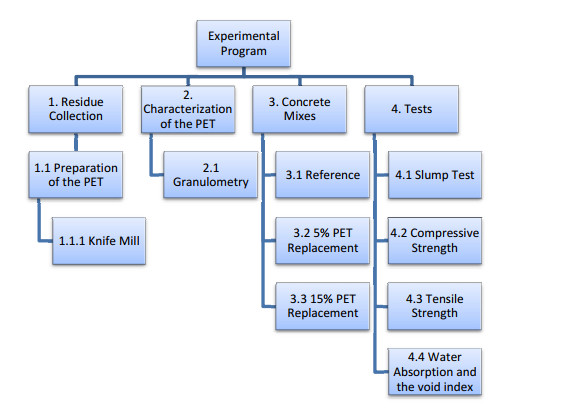
The expansion of cities contributed to the problems related to the accumulation of waste and lack of control over its management, there are still around 2400 dumps or uncontrolled landfills in Brazil. There is a large volume of polyethylene terephthalate (PET) improperly discarded. In turn, the construction industry has been looking for sustainable ways to produce concrete. This work deals with the analysis of the replacement of PET as a fine aggregate in concrete in the proportions of 5% and 15%. PET particles pass more than 75% in the 2.36 mm opening sieve and have more than 99% of their particle size retained in the 0.15 mm opening sieve. Concrete properties, compressive strength, tensile strength, water absorption and void ratio were evaluated and compared with the reference mix. In total, 45 specimens cast in concrete were used to complete the experiment. The results obtained showed that mixture compositions that incorporate PET as fine aggregates decrease compressive and tensile strength, increase water absorption and void index. The results obtained showed that blending compositions that incorporate PET as fine aggregates decrease compressive strength in about 14%, decrease tensile strength in about 7–11%, increased the void ratio in almost 20% and increased the water absorption in about 30%.

Keywords:

Citation: Filipe Figueiredo, Pamela da Silva, Eriton R. Botero, Lino Maia. Concrete with partial replacement of natural aggregate by PET aggregate—An exploratory study about the influence in the compressive strength[J]. AIMS Materials Science, 2022, 9(2): 172-183. doi: 10.3934/matersci.2022011

Related Papers:

[1]	Emadidin Gahalla Mohmed Elmahdi, Jianfei Huang . Two linearized finite difference schemes for time fractional nonlinear diffusion-wave equations with fourth order derivative. AIMS Mathematics, 2021, 6(6): 6356-6376. doi: 10.3934/math.2021373
[2]	Fouad Mohammad Salama, Faisal Fairag . On numerical solution of two-dimensional variable-order fractional diffusion equation arising in transport phenomena. AIMS Mathematics, 2024, 9(1): 340-370. doi: 10.3934/math.2024020
[3]	Ajmal Ali, Tayyaba Akram, Azhar Iqbal, Poom Kumam, Thana Sutthibutpong . A numerical approach for 2D time-fractional diffusion damped wave model. AIMS Mathematics, 2023, 8(4): 8249-8273. doi: 10.3934/math.2023416
[4]	Junying Cao, Zhongqing Wang, Ziqiang Wang . Stability and convergence analysis for a uniform temporal high accuracy of the time-fractional diffusion equation with 1D and 2D spatial compact finite difference method. AIMS Mathematics, 2024, 9(6): 14697-14730. doi: 10.3934/math.2024715
[5]	Abdul-Majeed Ayebire, Saroj Sahani, Priyanka, Shelly Arora . Numerical study of soliton behavior of generalised Kuramoto-Sivashinsky type equations with Hermite splines. AIMS Mathematics, 2025, 10(2): 2098-2130. doi: 10.3934/math.2025099
[6]	Yanjie Zhou, Xianxiang Leng, Yuejie Li, Qiuxiang Deng, Zhendong Luo . A novel two-grid Crank-Nicolson mixed finite element method for nonlinear fourth-order sin-Gordon equation. AIMS Mathematics, 2024, 9(11): 31470-31494. doi: 10.3934/math.20241515
[7]	Fouad Mohammad Salama, Nur Nadiah Abd Hamid, Norhashidah Hj. Mohd Ali, Umair Ali . An efficient modified hybrid explicit group iterative method for the time-fractional diffusion equation in two space dimensions. AIMS Mathematics, 2022, 7(2): 2370-2392. doi: 10.3934/math.2022134
[8]	Ailing Zhu, Yixin Wang, Qiang Xu . A weak Galerkin finite element approximation of two-dimensional sub-diffusion equation with time-fractional derivative. AIMS Mathematics, 2020, 5(5): 4297-4310. doi: 10.3934/math.2020274
[9]	Din Prathumwan, Thipsuda Khonwai, Narisara Phoochalong, Inthira Chaiya, Kamonchat Trachoo . An improved approximate method for solving two-dimensional time-fractional-order Black-Scholes model: a finite difference approach. AIMS Mathematics, 2024, 9(7): 17205-17233. doi: 10.3934/math.2024836
[10]	Fouad Mohammad Salama, Nur Nadiah Abd Hamid, Umair Ali, Norhashidah Hj. Mohd Ali . Fast hybrid explicit group methods for solving 2D fractional advection-diffusion equation. AIMS Mathematics, 2022, 7(9): 15854-15880. doi: 10.3934/math.2022868

Abstract

1. Introduction

Fractional-order differential equations (FDM) have many applications in various fields of engineering and science, such as chemical and physical phenomena ^[2,3,4,5]. For instance, the fractional-order diffusion equation is used to describe anomalous diffusion phenomena in the transport process through disordered and complex systems including fractal media, fractional kinetic equations regarding slow diffusion, and movement of small molecular along the concentration space ^[6].

In this article, the two-dimensional (2-D) time-fractional sub-diffusion equation (FSDE) with the weak singularity at initial time $t = 0$ is considered as follows:

$\begin{equation} \frac{\partial^{\alpha}V}{\partial t^{\alpha}} = \frac{\partial^{2}V}{\partial x^{2}} +\frac{\partial^{2}V}{\partial y^{2}} +G(x, y, t), \end{equation}$

(1.1)

with subject to conditions

$\begin{equation*} \begin{split} V(x, y, 0) = \zeta_0(x, y), \end{split} \end{equation*}$

and

$\begin{equation*} \begin{split} &V(0, y, t) = \zeta_1(x, y, t), \; V(L, y, t) = \zeta_2(x, y, t), \\& V(x, 0, t) = \zeta_3(x, y, t), \; V(x, L, t) = \zeta_4(x, y, t), \\& 0\leq x, y\leq M, \; 0\leq t\leq N, \end{split} \end{equation*}$

where $\zeta_0$ , $\zeta_1$ , $\zeta_2$ , $\zeta_3$ , $\zeta_4$ are known functions and $\alpha \in (0, 1)$ .

The FSDE can be obtained from the anomalous diffusion system by replacing the time derivative with a fractional derivative $\alpha$ where $0 < \alpha < 1$ . The FSDE is an important class of fractional partial differential equations (PDEs), which is mainly used in the modeling of fractional random walk, the phenomenon of wave propagation, diffusion unification, etc. ^[7,8].

The Caputo derivative of order $\alpha$ is

$\begin{equation} _{0}^{C}D_{t}^{\alpha} f(x) = \frac{1}{\Gamma (1-\alpha)}\int_{0}^{t} \frac{f'(x)}{(t-x)^{\alpha}} dx. \end{equation}$

(1.2)

The Caputo derivative approximated using the $L1$ gives the accuracy $2-\alpha$ ^[9,10], but the presence of kernel $(t-x)^{\alpha}$ produces solutions for Eq (1.1) with the weak-singularity at initial time $t = 0$ , which increases the computation cost and give low convergence rate for the approximate methods on uniform meshes ^[11]. Therefore, to increase the convergence rate many researchers solved the FSDE using different high-order numerical methods. Based on the chronology, several numerical methods are proposed for the solution of 2-D time FSDE (1.1), for example, Cui ^[12] proposed high-order alternating direction implicit (ADI) method, and it is unconditionally stable and convergent with convergence order $O(\nu^{\alpha}+h_0^{4})$ . Zhuang and Liu ^[13] proposed an unconditionally stable and convergent implicit difference scheme. Zhang et al. ^[14] used the Crank-Nicolson-type compact ADI scheme and proved the unconditional stability and convergence having convergence order $O(\nu^{min[2-\frac{\alpha}{2}, 2\alpha]}+h_0{1}^{4}+h_0{2}^{4})$ in $H_0^{1}$ norm. Ji and Sun ^[15] used a high-order numerical scheme to solve (1.1), and proved convergence in $L_{1}(L_{\infty})$ -norm and unconditional stability by the energy method. Wang et al. ^[16] solved 2-D FSDE using C-N alternating direction implicit finite difference method (FDM), where the fractional derivative is discretized using Riemann-Liouville fractional definition and to improve its temporal accuracy they used the Richardson extrapolation algorithm. Also, they proved its unique solvability, unconditional stability, and convergence $O(\nu^{2\gamma} + h_0{x}^{4} + h_0{y}^{4})$ of the scheme. Zhai and Feng ^[17] presented three different compact schemes for a 2-D time-fractional diffusion equation. The Caputo fractional definition is used for fractional derivative. All the schemes are fourth-order accurate for space and second-order accurate for the time variable. The stability of all the schemes is analyzed using Fourier analysis, which shows that two schemes are unconditionally stable, and the third one is conditionally stable.

The advantage of high-order schemes is that it produces more accurate results but at the same time increase the execution timings because of the escalated computational complexity of the scheme. Similarly, the advantage of explicit group methods over the standard point methods that the it considered quarter grid points of the solution domain and the points are considered as iterative points in the iterative process which reduces the computational complexity of the proposed method and hence reduce the execution time per iteration. Since, the computational complexity is greatly reduced using the explicit group method the 2-D time-fractional advection-diffusion, hyperbolic telegraph fractional differential, and fractional diffusion equations etc. ^{[18,19,20,21,22]} with second-order accuracy, therefore, we proposed the grouping strategy with uniform grids for the solution of the 2-D time FSDE with fourth-order accuracy. The purpose of this paper is to solve 2-D time FSDE with the fourth-order explicit group method (FEGM).

The paper is organized as follows: In Section 2, the derivation of the group explicit method from the finite difference method is presented. Section 3 discussed the stability of the proposed scheme, and the convergence of the proposed scheme is presented in Section 4. To show the efficiency of the proposed method, some numerical examples with discussion are presented in Section 5, and finally, Section 6 consists of the conclusion.

2. The fourth-order grouping scheme

First, let us define some notations:

$\begin{equation*} \begin{split} &\delta_{x}^2 V_{i, j}^{k} = V_{i+1, j}^{k}- 2 V_{i, j}^{k} + V_{i-1, j}^{k}, \; V_{i, j}^{k + \frac{1}{2} } = \frac{V_{i, j}^{k+1} + V_{i, j}^{k} }{2}, \\ & x_{i} = i h_0, \; y_{j} = j h_0, \; i, j = 0, 1, 2, 3..., M, \\ & t_{k} = k \nu, \; k = 0, 1, 2, 3..., N, \end{split} \end{equation*}$

where $h_0 = \Delta x = \Delta y = \frac{L}{M}$ represents the space step and $\nu = \frac{T}{N}$ time step.

Since, the Taylor series expansion with respect to $x$ is

$\begin{equation} V_{i+1, j}^{k} = V_{i, j}^{k}+ \frac{h_0}{1!}V_{x}|_{i, j}^{k} + \frac{h_0^{2}}{2!}V_{xx}|_{i, j}^{k} + \frac{h_0^{3}}{3!}V|_{i, j}^{k} + ..., \end{equation}$

(2.1)

$\begin{equation} V_{i-1, j}^{k} = V_{i, j}^{k}- \frac{h_0}{1!} V_{x}|_{i, j}^{k} + \frac{h_0^{2}}{2!} V_{xx}|_{i, j}^{k} - \frac{h_0^{3}}{3!} V_{xxx}|_{i, j}^{k} + ... \end{equation}$

(2.2)

By adding Eqs (2.1) and (2.2) and after rearranging, we get

$\begin{equation} \begin{split} \frac{\partial^2 V_{i, j}^{k}}{\partial x^2}& = \frac{V_{i+1, j}^{k}-2u_{i, j}^{k}+V_{i-1, j}^{k}}{h_0^{2}} + \frac{2h_0^{2}}{4!}\frac{\partial^4 V_{i, j}^{k} }{\partial x^4} +...\\& = \frac{V_{i+1, j}^{k}-2V_{i, j}^{k}+V_{i-1, j}^{k}}{h_0^{2}} + O(h_0^{2}). \end{split} \end{equation}$

(2.3)

Therefore, the Taylor series expansions at points $u_{i+1, j}^{k}$ and $u_{i, j+1}^{k}$ are

$\begin{equation} \frac{\delta^{2}_{x}}{h_{0}^2} V_{i, j}^{k} = \frac{\partial^2 V}{\partial x^2}|_{i, j}^{k} - \frac{h_{0}^{2}}{12}\frac{\partial^4 V}{\partial x^4}|_{i, j}^{k} - \frac{h_{0}^{4}}{360}\frac{\partial^6 V}{\partial x^6}|_{i, j}^{k} + O(h_0^{6}), \end{equation}$

(2.4)

$\begin{equation} \frac{\delta^{2}_{y}}{h_{0}^2} V_{i, j}^{k} = \frac{\partial^2 V}{\partial y^2}|_{i, j}^{k} - \frac{h_{0}^{2}}{12}\frac{\partial^4 V}{\partial y^4}|_{i, j}^{k} + \frac{h_{0}^{4}}{360}\frac{\partial^6 V}{\partial y^6}|_{i, j}^{k} + O(h_0^{6}). \end{equation}$

(2.5)

The difference operator $\delta_{x}^2$ , which maintain the three-point stencil is given by ^[]

$\begin{equation} \begin{split} \frac{\delta_{x}^{2}}{h_0^{2}(1+\frac{1}{12}\delta _{x}^{2})} V_{i, j}^{k} = \left.\begin{matrix} \frac{\partial^{2}V}{\partial x^{2}} \end{matrix}\right|_{i, j}^{k}-\frac{h_0^{4}}{240}\left.\begin{matrix} \frac{\partial^{4 }V}{\partial x^{4}} \end{matrix}\right|_{i, j}^{k} + O(h_0^{6}), \end{split} \end{equation}$

(2.6)

and

$\begin{equation} \begin{split} \frac{\delta_{y}^{2}}{h_0^{2}(1+\frac{1}{12}\delta _{y}^{2})} V_{i, j}^{k} = \left.\begin{matrix} \frac{\partial^{2}V}{\partial y^{2}} \end{matrix}\right|_{i, j}^{k}-\frac{h_0^{4}}{240}\left.\begin{matrix} \frac{\partial^{4 }V}{\partial y^{4}} \end{matrix}\right|_{i, j}^{k} + O(h_0^{6}). \end{split} \end{equation}$

(2.7)

The fractional derivative is approximated using the Central difference formula as ^[24]

$\begin{equation*} \begin{split} \frac{\partial^\alpha }{\partial t^\alpha} V(x, y, t)|_{i, j}^{k+\frac{1}{2}} = &\frac{1}{\Gamma (1-\alpha)}\int_{0}^{t_{k+\frac{1}{2}}}V_t(x, y, \varepsilon) (t_{k+\frac{1}{2}}-\varepsilon)^{-\alpha}\partial\varepsilon \\ = &\frac{1}{\Gamma (1-\alpha)}\left [ \int_{0}^{t_{k+\frac{1}{2}}}V_t(x, y, \varepsilon) \left((k+\frac{1}{2}) \nu-\varepsilon\right)^{-\alpha}\partial\varepsilon \right.\\& \left. + \int_{t_k}^{t_{t_{k+\frac{1}{2}}}}\left (\frac{V_{i, j}^{k+1}-V_{i, j}^k}{\nu} + O (\nu)\right ) \left((k+\frac{1}{2})\nu-\varepsilon\right)^{-\alpha}\partial\varepsilon \right ] \\ = &\frac{1}{\Gamma (1-\alpha)} \sum\limits_{s_0 = 1}^{k}\left [ \int_{(s_0-1)\nu}^{s\nu} \frac{V_{i, j}^{s_0} -V_{i, j}^{s_0-1}}{\nu} + (\varepsilon -t_{s_0-\frac{1}{2}})V_{tt}(x_i, y_j, c_{s_0}) \right.\\& \times \left. ((k+\frac{1}{2}\nu-\varepsilon)^{-\alpha}\partial\varepsilon )\right ] + \int_{k\nu}^{(k+\frac{1}{2})\nu}\left ( \frac{V_{i, j}^{k+1}-V_{i, j}^k}{\nu} + O (\nu)\right ) \left((k+\frac{1}{2})\nu-\varepsilon\right)^{-\alpha}\partial\varepsilon \\ = &\frac{1}{\Gamma (1-\alpha)} \sum\limits_{s_0 = 1}^{k} \frac{V_{i, j}^{s_0} -V_{i, j}^{s_0-1}}{\nu} \int_{(s_0-1)\nu}^{s\nu} \left((k+\frac{1}{2})\nu - \varepsilon \right)^{-\alpha}\partial \varepsilon \\& + \frac{1}{\Gamma (1-\alpha)} \sum\limits_{s_0 = 1}^{k} \int_{(s-1)\nu}^{s\nu} (\varepsilon -t_{s_0 -\frac{1}{2}})V_{tt}(x_i, y_j, c_{s_0}) \left ((k+\frac{1}{2})\nu-\varepsilon\right)^{-\alpha}\partial\varepsilon \\& +\frac{1}{\Gamma(1-\alpha)} \left [ \frac{V_{i, j}^{k+1}-V_{i, j}^{k}}{\nu} +O(\nu)\right ] \int_{k\nu}^{(k+\frac{1}{2})\nu} \left[ \left((k+\frac{1}{2})\nu-\varepsilon \right)^{-\alpha}-\varepsilon \right]\partial \varepsilon \\ = &\frac{1}{\nu^\alpha (1-\alpha)\Gamma (1-\alpha) } \sum\limits_{s_0 = 1}^{k} \left [V_{i, j}^{s_0} -V_{i, j}^{s_0-1} \right ] \left [ (k-s_0+\frac{3}{2})^{1-\alpha} -(k-s_0+\frac{1}{2})^{1-\alpha} \right ] \\& + \frac{1}{\nu^\alpha (1-\alpha) \Gamma (1-\alpha) } (V_{i, j}^{k+1}-V_{i, j}^{k})\frac{1}{2^{1-\alpha}} \\& + \frac{1}{\Gamma (1-\alpha)} \sum\limits_{s_0 = 1}^{k} \int_{(s-1)\nu}^{s\nu} (\varepsilon -t_{s_0 -\frac{1}{2}})V_{tt}(x_i, y_j, c_{s_0}) \left((k+\frac{1}{2})\nu-\varepsilon \right)^{-\alpha}\partial\varepsilon \\& + \frac{1}{\Gamma (1-\alpha)(1-\alpha)2^{1-\alpha}}O(\nu)^{2-\alpha}. \end{split} \end{equation*}$

Therefore, after some simplifications, the Crank-Nicolson (C-N) Caputo fractional derivative

$\begin{equation} \begin{array}{c} \frac{\partial^{\alpha} }{\partial t^{\alpha}}\left.\begin{matrix} V(x, y, t) \end{matrix}\right|_{i, j}^{k+\frac{1}{2}} = a_{1}\left.\begin{matrix} V \end{matrix}\right|_{i, j}^{k}+\sum\limits_{s = 1}^{k-1}(a_{k-s+1}-a_{k-s}) \left.\begin{matrix} V \end{matrix}\right|_{i, j}^{s} -a_{k} \left.\begin{matrix} V \end{matrix}\right|_{i, j}^{0}+ \sigma \frac{V_{i, j}^{k+1}+V_{i, j}^{k}}{2^{1-\alpha}}+O(\nu^{2-\alpha}),\\ \sigma = \frac{1}{\nu^{\alpha}\Gamma(2-\alpha)}, \; a_{s} = \sigma\left( (s+\frac{1}{2})^{1-\alpha}-(s-\frac{1}{2})^{1-\alpha} \right), \; s = 0, 1, 2, ..., k. \end{array}\end{equation}$

(2.8)

Now using Eqs (2.6)–(2.8) and C-N or standard point (SP) scheme at $V(x_{i}, y_{j}, t_{k+\frac{1}{2}})$ , the standard fourth-order finite difference scheme for Eq (1.1) is as follows:

$\begin{equation} \begin{split} &a_{1}V_{i, j}^{k}+\sum\limits_{s = 1}^{k-1}(a_{k-s+1}-a_{k-s})V_{i, j}^{s}-a_{k}V_{i, j}^{0}+\sigma\frac{V_{i, j}^{k+1}+V_{i, j}^{k}}{2^{1-\alpha}}\\ = &\left( 1+\frac{1}{12}\delta_{x}^{2} \right)^{-1} \times \frac{\delta_{x}^{2}}{h_0^{2}}V_{i, j}^{k+\frac{1}{2}} +\left( 1+\frac{1}{12}\delta_{y}^{2} \right)^{-1} \frac{\delta_{y}^{2}}{h_0^{2}}V_{i, j}^{k+\frac{1}{2}} + f_{i, j}^{k+\frac{1}{2}} + O(\nu^{2-\alpha}+h_0^{4}). \end{split} \end{equation}$

(2.9)

Substituting the values of $\delta_{x}^{2}$ , $\delta_{y}^{2}$ and $V_{i, j}^{k+\frac{1}{2}}$ into Eq (2.9), and after rearranging we get the standard point SP compact scheme:

$\begin{equation} \begin{split} \lambda_{1}V_{i, j}^{k+1} = & \lambda_{2}(V_{i+1, j}^{k+1}+ V_{i-1, j}^{k+1}+ V_{i, j+1}^{k+1}+V_{i, j-1}^{k+1})+\lambda_{3}(V_{i+1, j+1}^{k+1}+ V_{i-1, j+1}^{k+1} \\& +V_{i+1, j-1}^{k+1}+V_{i-1, j-1}^{k+1})+\lambda_{4}V_{i, j}^{k}+\lambda_{5}(V_{i+1, j}^{k}+ V_{i-1, j}^{k}+ V_{i, j+1}^{k} \\ & +V_{i, j-1}^{k})+\lambda_{6}(V_{i+1, j+1}^{k}+ V_{i-1, j+1}^{k}+ V_{i+1, j-1}^{k}+V_{i-1, j-1}^{k}) \\& +\frac{25}{18}h_{0}^{2}f_{i, j}^{k+\frac{1}{2}}+\frac{5}{36}h_{0}^{2}(f_{i+1, j}^{k+\frac{1}{t}}+f_{i-1, j}^{k+\frac{1}{t}}+f_{i, j+1}^{k+\frac{1}{t}}+f_{i, j-1}^{k+\frac{1}{t}}) \\& +\frac{h_{0}^{2}}{72}(f_{i+1, j+1}^{k+\frac{1}{2}}+f_{i-1, j+1}^{k+\frac{1}{2}}+f_{i+1, j-1}^{k+\frac{1}{2}}+f_{i-1, j-1}^{k+\frac{1}{2}}) \\& -\sum\limits_{s = 1}^{k-1}(a_{k-s+1}-a_{k-s}) \left(\frac{25}{18}h_0^{2}V_{i, j}^{s}+\frac{5}{36}h_0^{2}(V_{i+1, j}^{s}+V_{i-1, j}^{s}+V_{i, j+1}^{s} \right. \\& \left. +V_{i, j-1}^{s})+\frac{h_0^{2}}{72}(V_{i+1, j+1}^{s}+V_{i-1, j+1}^{s}+V_{i+1, j-1}^{s}+V_{i-1, j-1}^{s})\right) + O(\nu^{2-\alpha}+h_0^{4}), \end{split} \end{equation}$

(2.10)

where

$\begin{equation*} \begin{split} &g_0 = \frac{\sigma}{2^{1-\alpha}}, \; g_1 = a_{1}-g_0, \; \lambda_{1} = \frac{1}{72}(240+100h_0^{2}g_0), \; \lambda_{2} = \frac{1}{72}(48-10h_0^{2}g_0), \; \\& \lambda_{3} = \frac{1}{72}(12-h_0^{2}g_0), \; \lambda_{4} = -\frac{1}{72}(240+100h_0^{2}g_1), \; \lambda_{5} = \frac{1}{72}(48-10h_0^{2}g_1), \; \\& \lambda_{6} = \frac{1}{72}(12-h_0^{2}g_1). \end{split} \end{equation*}$

Now, using Eq (2.10) will give the following system for the group of four points:

$\begin{equation} \begin{bmatrix} \lambda_{1} & -\lambda_{2} & -\lambda_{3} & -\lambda_{2}\\ -\lambda_{2}&\lambda_{1} & -\lambda_{2} & -\lambda_{3} \\ -\lambda_{3}& -\lambda_{2} & \lambda_{1} & -\lambda_{2} \\ -\lambda_{2}& -\lambda_{3} & -\lambda_{2} & \lambda_{1} \end{bmatrix} \begin{bmatrix} V_{i, j}^{k+1}\\ V_{i+1, j}^{k+1}\\ V_{i+1, j+1}^{k+1}\\ V_{i, j+1}^{k+1} \end{bmatrix} = \begin{bmatrix} rhs_{i, j}\\ rhs_{i+1, j}\\ rhs_{i+1, j+1}\\ rhs_{i, j+1} \end{bmatrix}, \end{equation}$

(2.11)

where

$\begin{equation*} \begin{split} rhs_{i, j} = & \lambda_{2}(V_{i-1, j}^{k+1}+V_{i, j-1}^{k+1})+\lambda_{3} (V_{i-1, j+1}^{k+1}+V_{i+1, j-1}^{k+1}+V_{i-1, j-1}^{k+1})+\lambda_{4}V_{i, j}^{k}\\& +\lambda_{5}(V_{i+1, j}^{k}+V_{i-1, j}^{k}+V_{i, j+1}^{k}+V_{i, j-1}^{k})+\lambda_{6}(V_{i+1, j+1}^{k}+V_{i-1, j+1}^{k} \\& +V_{i+1, j-1}^{k}+V_{i-1, j-1}^{k})+\frac{25}{18}h_0^{2}f_{i, j}^{k+\frac{1}{2}}+\frac{5}{36}h_0^{2}(f_{i+1, j}^{k+\frac{1}{2}}+f_{i-1, j}^{k+\frac{1}{2}}+f_{i, j+1}^{k+\frac{1}{2}} \\& +f_{i, j-1}^{k+\frac{1}{2}})+ \frac{h_0^{2}}{72}(f_{i+1, j+1}^{k+\frac{1}{2}}+f_{i-1, j+1}^{k+\frac{1}{2}}+f_{i+1, j-1}^{k+\frac{1}{2}}+f_{i-1, j-1}^{k+\frac{1}{2}}) - F_{i, j}, \end{split} \end{equation*}$

$\begin{equation*} \begin{split} rhs_{i+1, j} = & \lambda_{2}(V_{i+2, j}^{k+1}+V_{i+1, j-1}^{k+1})+\lambda_{3} (V_{i+2, j+1}^{k+1}+V_{i+2, j-1}^{k+1}+V_{i, j-1}^{k+1})+\lambda_{4} V_{i+1, j}^{k}\\& +\lambda_{5}(V_{i+2, j}^{k}+V_{i, j}^{k}+V_{i+1, j+1}^{k}+V_{i+1, j-1}^{k})+\lambda_{6}(V_{i+2, j+1}^{k}+V_{i, j+1}^{k} \\& +V_{i+2, j-1}^{k}+V_{i, j-1}^{k})+\frac{25}{18}h_0^{2}f_{i+1, j}^{k+\frac{1}{2}}+\frac{5}{36}h_0^{2}(f_{i+2, j}^{k+\frac{1}{2}}+f_{i, j}^{k+\frac{1}{2}}+f_{i+1, j+1}^{k+\frac{1}{2}} \\& +f_{i+1, j-1}^{k+\frac{1}{2}})+ \frac{h_0^{2}}{72}(f_{i+2, j+1}^{k+\frac{1}{2}}+f_{i, j+1}^{k+\frac{1}{2}}+f_{i+2, j-1}^{k+\frac{1}{2}}+f_{i, j-1}^{k+\frac{1}{2}})- F_{i+1, j}, \end{split} \end{equation*}$

$\begin{equation*} \begin{split} rhs_{i+1, j+1} = & \lambda_{2}(V_{i+2, j+1}^{k+1}+V_{i+1, j+2}^{k+1})+\lambda_{3} (V_{i+2, j+2}^{k+1}+V_{i, j+2}^{k+1}+V_{i+2, j}^{k+1})+\lambda_{4} V_{i+1, j+1}^{k}\\& +\lambda_{5}(V_{i+2, j+1}^{k}+V_{i, j+1}^{k}+V_{i+1, j+2}^{k}+V_{i+1, j}^{k})+\lambda_{6}(V_{i+2, j+2}^{k}+V_{i, j+2}^{k} \\& +V_{i+2, j}^{k}+V_{i, j}^{k})+\frac{25}{18}h_0^{2}f_{i+1, j+1}^{k+\frac{1}{2}}+\frac{5}{36}h_0^{2}(f_{i+2, j+1}^{k+\frac{1}{2}}+f_{i, j+1}^{k+\frac{1}{2}}+f_{i+1, j+2}^{k+\frac{1}{2}} \\& +f_{i+1, j}^{k+\frac{1}{2}})+ \frac{h_0^{2}}{72}(f_{i+2, j+2}^{k+\frac{1}{2}}+f_{i, j+2}^{k+\frac{1}{2}}+f_{i+2, j}^{k+\frac{1}{2}}+f_{i, j}^{k+\frac{1}{2}})- F_{i+1, j+1}, \end{split} \end{equation*}$

$\begin{equation*} \begin{split} rhs_{i, j+1} = & \lambda_{2}(V_{i-1, j+1}^{k+1}+V_{i, j+2}^{k+1})+\lambda_{3} (V_{i+1, j+2}^{k+1}+V_{i-1, j+2}^{k+1}+V_{i-1, j}^{k+1})+\lambda_{4}V_{i, j+1}^{k}\\& +\lambda_{5}(V_{i+1, j+1}^{k}+V_{i-1, j+1}^{k}+V_{i, j+2}^{k}+V_{i, j}^{k})+\lambda_{6}(V_{i+1, j+2}^{k}+V_{i-1, j+2}^{k} \\& +V_{i+1, j}^{k}+V_{i-1, j}^{k})+\frac{25}{18}h_0^{2}f_{i, j+1}^{k+\frac{1}{2}}+\frac{5}{36}h_0^{2}(f_{i+1, j+1}^{k+\frac{1}{2}}+f_{i-1, j+1}^{k+\frac{1}{2}}+f_{i, j+2}^{k+\frac{1}{2}} \\& +f_{i, j}^{k+\frac{1}{2}})+ \frac{h_0^{2}}{72}(f_{i+1, j+2}^{k+\frac{1}{2}}+f_{i-1, j+2}^{k+\frac{1}{2}}+f_{i+1, j}^{k+\frac{1}{2}}+f_{i-1, j}^{k+\frac{1}{2}})- F_{i, j+1}, \end{split} \end{equation*}$

and

$\begin{equation*} \begin{split} F_{i, j} = &\sum\limits_{s = 1}^{k-1}(a_{k-s+1}-a_{k-s}) \left(\frac{25}{18}h_0^{2}V_{i, j}^{s}+\frac{5}{36}h_0^{2}(V_{i+1, j}^{s}+V_{i-1, j}^{s}+V_{i, j+1}^{s} \right. \\& \left. +V_{i, j-1}^{s})+\frac{h_0^{2}}{72}(V_{i+1, j+1}^{s}+V_{i-1, j+1}^{s}+V_{i+1, j-1}^{s}+V_{i-1, j-1}^{s})\right). \end{split} \end{equation*}$

Similarly, the inverted matrix equation (2.11) will give explicit group equation

$\begin{equation} \begin{bmatrix} V_{i, j}^{k+1}\\ V_{i+1, j}^{k+1}\\ V_{i+1, j+1}^{k+1}\\ V_{i, j+1}^{k+1} \end{bmatrix} = \frac{1}{d}\begin{bmatrix} \phi_{1} & \phi_{2} & \phi_{3} & \phi_{2} \\ \phi_{2} & \phi_{1} & \phi_{2} & \phi_{3} \\ \phi_{3} & \phi_{2} & \phi_{1} & \phi_{2} \\ \phi_{2} & \phi_{3} & \phi_{2} & \phi_{1} \end{bmatrix} \begin{bmatrix} rhs_{i, j}\\ rhs_{i+1, j}\\ rhs_{i+1, j+1}\\ rhs_{i, j+1} \end{bmatrix}, \end{equation}$

(2.12)

where

$\begin{equation*} \begin{split} &\phi_{1} = \lambda_{1}^{3}-2\lambda_{1}\lambda_{2}^{2}-2\lambda_{2}^{2}\lambda_{3}-\lambda_{1}\lambda_{3}^{2}, \; \phi_{2} = \lambda_{1}^{2}\lambda_{2}+2\lambda_{1}\lambda_{2}\lambda_{3}+\lambda_{2}\lambda_{3}^{2}, \\& \phi_{3} = 2\lambda_{1}\lambda_{2}^{2}+\lambda_{1}^{2}\lambda_{3}+2\lambda_{2}^{2}\lambda_{3}-\lambda_{3}^{3}, \; d = (-4\lambda_{2}^{2}+(\lambda_{1}-\lambda_{3})^{2})(\lambda_{1}+\lambda_{3})^{2}. \end{split} \end{equation*}$

In the proposed method, firstly, group of four points are computed for the different iterations using Eq (2.12) till the required convergence is attained. After the required convergence, the SP compact scheme Eq (2.10) is used directly once for computing of reaming points. and show the grid points on the x-y plane for FDM and FEGM at various time levels when $m = 9$ respectively.

Figure 1. Four points in computation of grouping method.

DownLoad: Full-Size Img PowerPoint

Figure 2. Different points in the FEGM at time levels

$k + 1, k, k-1, ..., 1$ with mesh size

$m = 9$ .

DownLoad: Full-Size Img PowerPoint

3. Stability of the FEGM

In this section, the stability of the proposed method is discussed.

The Eq (2.12) can also be written as

$\begin{equation} \begin{split} & AV^{1} = BV^{0}+f^{\frac{1}{2}}, \; k = 0, \\& AV^{k+1} = BV^{k}-h_0^{2}\sum\limits_{s = 1}^{k-1}(a_{k-s+1}-a_{k-s})CV^{s}+h_0^{2}f^{k+\frac{1}{2}}, \; k > 0, \end{split} \end{equation}$

(3.1)

where

$\begin{equation*} \begin{split} &A = \begin{bmatrix} R_{1} & R_{3} & & & 0\\ R_{2}& R_{1} & R_{3} & & \\ & R_{2} & R_{1} & & \\ & & & \ddots & R_{3}\\ 0 & & &R_{2} & R_{1} \end{bmatrix}, \; B = \begin{bmatrix} P_{1} & P_{3} & & & 0\\ P_{2}& P_{1} & P_{3} & & \\ & P_{2} & P_{1} & & \\ & & & \ddots & P_{3}\\ 0 & & &P_{2} & P_{1} \end{bmatrix}, \end{split} \end{equation*}$

$\begin{equation*} \begin{split} &R_{1} = \begin{bmatrix} G_{1} & G_{3} & & & \\ G_{2}& G_{1} & G_{3} & & \\ & G_{2} & G_{1} & & \\ & & & \ddots & G_{3}\\ & & &G_{2} & G_{1} \end{bmatrix}, \; C = \begin{bmatrix} Q_{1} & Q_{3} & & & 0\\ Q_{2}& Q_{1} & Q_{3} & & \\ & Q_{2} & Q_{1} & & \\ & & & \ddots & Q_{3}\\ 0 & & &Q_{2} & Q_{1} \end{bmatrix}, \; f = \begin{bmatrix} K_1\\ K_1\\ \vdots \\ K_1\\ K_1 \end{bmatrix}, \end{split} \end{equation*}$

$\begin{equation*} R_{2} = \begin{bmatrix} G_{6} & G_{4} & & & \\ G_{8}& G_{6} & G_{4} & & \\ & G_{8} & G_{6} & & \\ & & & \ddots & G_{4}\\ & & &G_{8} & G_{6} \end{bmatrix}, \; R_{3} = \begin{bmatrix} G_{7} & G_{9} & & & \\ G_{5}& G_{7} & G_{9} & & \\ & G_{5} & G_{7} & & \\ & & & \ddots & G_{9}\\ & & &G_{5} & G_{7} \end{bmatrix}, \end{equation*}$

$\begin{equation*} \begin{split} P_{1} = \begin{bmatrix} H_{1} & H_{3} & & & \\ H_{2}& H_{1} & H_{3} & & \\ & H_{2} & H_{1} & & \\ & & & \ddots & H_{3}\\ & & &H_{2} & H_{1} \end{bmatrix}, \; P_{2} = \begin{bmatrix} H_{6} & H_{4} & & & \\ H_{8}& H_{6} & H_{4} & & \\ & H_{8} & H_{6} & & \\ & & & \ddots & H_{4}\\ & & &H_{8} & H_{6} \end{bmatrix}, \end{split} \end{equation*}$

$\begin{equation*} P_{3} = \begin{bmatrix} H_{7} & H_{9} & & & \\ H_{5}& H_{7} & H_{9} & & \\ & H_{5} & H_{7} & & \\ & & & \ddots & H_{9}\\ & & &H_{5} & H_{7} \end{bmatrix}, \; Q_{1} = \begin{bmatrix} L_{1} & L_{3} & & & \\ L_{2}& L_{1} & L_{3} & & \\ & L_{2} & L_{1} & & \\ & & & \ddots & L_{3}\\ & & &L_{2} & L_{1} \end{bmatrix}, \end{equation*}$

$\begin{equation*} Q_{2} = \begin{bmatrix} L_{6} & L_{4} & & & \\ L_{8}& L_{6} & L_{4} & & \\ & L_{8} & L_{6} & & \\ & & & \ddots & L_{4}\\ & & &L_{8} & L_{6} \end{bmatrix}, \; Q_{3} = \begin{bmatrix} L_{7} & L_{9} & & & \\ L_{5}& L_{7} & L_{9} & & \\ & L_{5} & L_{7} & & \\ & & & \ddots & L_{9}\\ & & &L_{5} & L_{7} \end{bmatrix}, \; K_1 = \begin{bmatrix} W_1\\ W_1\\ \vdots \\ W_1\\ W_1 \end{bmatrix}, \end{equation*}$

$\begin{equation*} G_{1} = \begin{bmatrix} \lambda_{1} & -\lambda_{2} & -\lambda_{3} & -\lambda_{2}\\ -\lambda_{2}&\lambda_{1} & -\lambda_{2} & -\lambda_{3} \\ -\lambda_{3}& -\lambda_{2} & \lambda_{1} & -\lambda_{2} \\ -\lambda_{2}& -\lambda_{3} & -\lambda_{2} & \lambda_{1} \end{bmatrix}, \; G_{2} = \begin{bmatrix} 0 & 0 & -\lambda_{3} & -\lambda_{2}\\ 0&0 & -\lambda_{2} & -\lambda_{3} \\ 0& 0 &0 & 0 \\ 0& 0 &0 & 0 \end{bmatrix}, \; G_{3} = \begin{bmatrix} 0 & 0 & 0& 0\\ 0&0 & 0 & 0 \\ -\lambda_{3}& -\lambda_{2} &0 & 0 \\ -\lambda_{2}& -\lambda_{3} &0 & 0 \end{bmatrix}, \end{equation*}$

$\begin{equation*} G_{4} = \begin{bmatrix} 0 & 0 & 0& 0\\ 0&0 & 0 & 0 \\ 0& 0 &0 & 0 \\ 0& -\lambda_{3} &0 & 0 \end{bmatrix}, \; G_{5} = \begin{bmatrix} 0 & 0 & 0& 0\\ 0&0 & 0 & -\lambda_{3} \\ 0& 0 &0 & 0 \\ 0& 0 &0 & 0 \end{bmatrix}, \; G_{6} = \begin{bmatrix} 0 & -\lambda_{2}& -\lambda_{3}& 0\\ 0&0 & 0 & 0 \\ 0& 0 &0 & 0 \\ 0& -\lambda_{3} &-\lambda_{2} & 0 \end{bmatrix}, \end{equation*}$

$\begin{equation*} G_{7} = \begin{bmatrix} 0 & 0& 0& 0\\ -\lambda_{2}&0 & 0 & -\lambda_{3}\\ -\lambda_{3}& 0 &0 & -\lambda_{2} \\ 0&0 &0 & 0 \end{bmatrix}, \; G_{8} = \begin{bmatrix} 0 & 0& -\lambda_{3}& 0\\ 0&0 & 0 & 0\\ 0& 0 &0 & 0 \\ 0&0 &0 & 0 \end{bmatrix}, \; G_{9} = \begin{bmatrix} 0 & 0& 0& 0\\ 0&0 & 0 & 0\\ -\lambda_{3}& 0 &0 & 0 \\ 0&0 &0 & 0 \end{bmatrix}, \end{equation*}$

$\begin{equation*} H_{1} = \begin{bmatrix} \lambda_{4} & \lambda_{5} & \lambda_{6} & \lambda_{5}\\ \lambda_{5}&\lambda_{4} & \lambda_{5} & \lambda_{6} \\ \lambda_{6}& \lambda_{5} & \lambda_{4} & \lambda_{5} \\ \lambda_{5}& \lambda_{6} & \lambda_{5} & \lambda_{4} \end{bmatrix}, \; H_{2} = \begin{bmatrix} 0 & 0 & \lambda_{6} & \lambda_{5}\\ 0&0 & \lambda_{5} & \lambda_{6} \\ 0& 0 &0 & 0 \\ 0& 0 &0 & 0 \end{bmatrix}, \; H_{3} = \begin{bmatrix} 0 & 0 & 0 & 0\\ 0&0 & 0 & 0\\ \lambda_{6}& \lambda_{5} &0 & 0 \\ \lambda_{5}& \lambda_{6} &0 & 0 \end{bmatrix}, \end{equation*}$

$\begin{equation*} \begin{split} & H_{4} = \begin{bmatrix} 0 & 0 & 0 & 0\\ 0&0 & 0 & 0\\ 0& 0 &0 & 0 \\ 0& \lambda_{6} &0 & 0 \end{bmatrix}, \; H_{5} = \begin{bmatrix} 0 & 0 & 0 & 0\\ 0&0 & 0 & \lambda_{6}\\ 0& 0 &0 & 0 \\ 0& 0 &0 & 0 \end{bmatrix}, \; H_{6} = \begin{bmatrix} 0 & \lambda_{5} & \lambda_{6} & 0\\ 0&0 & 0 & 0\\ 0& 0 &0 & 0 \\ 0& \lambda_{6} &\lambda_{5} & 0 \end{bmatrix}, \\ \end{split} \end{equation*}$

$\begin{equation*} H_{7} = \begin{bmatrix} 0 & 0 & 0& 0\\ \lambda_{5} &0 & 0 & \lambda_{6} \\ \lambda_{6} & 0 &0 & \lambda_{5} \\ 0& 0&0 & 0 \end{bmatrix}, \; H_{8} = \begin{bmatrix} 0 & 0 & \lambda_{6}& 0\\ 0 &0 & 0 & 0 \\ 0 & 0 &0 & 0 \\ 0& 0&0 & 0 \end{bmatrix}, \; H_{9} = \begin{bmatrix} 0 & 0 & 0& 0\\ 0 &0 & 0 & 0 \\ \lambda_{6} & 0 &0 & 0 \\ 0& 0&0 & 0 \end{bmatrix}, \end{equation*}$

$\begin{equation*} L_{1} = \frac{1}{18}\begin{bmatrix} 25 & \frac{5}{2} & \frac{1}{4} & \frac{5}{4}\\ \frac{5}{2} & 25 & \frac{5}{2}& \frac{1}{4}\\ \frac{1}{4}& \frac{5}{2} & 25 & \frac{5}{2}\\ \frac{5}{2}&\frac{1}{4} & \frac{5}{2} & 25 \end{bmatrix}, \; L_{2} = \frac{1}{18}\begin{bmatrix} 0 & 0 & \frac{1}{4} & \frac{5}{4}\\ 0 & 0 & \frac{5}{2}& \frac{1}{4}\\ 0& 0 & 0 & 0\\ 0&0 & 0 &0 \end{bmatrix}, \; L_{3} = \frac{1}{18}\begin{bmatrix} 0 & 0 & 0 & 0\\ 0 & 0 & 0& 0\\ \frac{1}{4}& \frac{5}{4} & 0 & 0\\ \frac{5}{4}&\frac{1}{4} & 0 &0 \end{bmatrix}, \end{equation*}$

$\begin{equation*} L_{4} = \begin{bmatrix} 0 & 0 & 0 & 0\\ 0 & 0 & 0& 0\\ 0& 0 & 0 & 0\\ 0&\frac{1}{72} & 0 &0 \end{bmatrix}, \; L_{5} = \begin{bmatrix} 0 & 0 & 0 & 0\\ 0 & 0 & 0& \frac{1}{72}\\ 0& 0 & 0 & 0\\ 0& 0& 0 &0 \end{bmatrix}, \; L_{6} = \frac{1}{18}\begin{bmatrix} 0 & \frac{5}{2} & \frac{1}{4} & 0\\ 0 & 0 & 0& 0\\ 0& 0 & 0 & 0\\ 0& \frac{1}{4}& \frac{5}{2}&0 \end{bmatrix}, \end{equation*}$

$\begin{equation*} \begin{split} & L_{7} = \frac{1}{18}\begin{bmatrix} 0 & 0 & 0 & 0\\ \frac{5}{2} & 0 & 0&\frac{1}{4}\\ \frac{1}{4}& 0 & 0 & \frac{5}{2}\\ 0& 0& 0&0 \end{bmatrix}, \; L_{8} = \begin{bmatrix} 0 & 0 & \frac{1}{72} & 0\\ 0 & 0 & 0&0\\ 0& 0 & 0 &0\\ 0& 0& 0&0 \end{bmatrix}, \; L_{9} = \begin{bmatrix} 0 & 0 & 0 & 0\\ 0 & 0 & 0&0\\ \frac{1}{72}& 0 & 0 &0\\ 0& 0& 0&0 \end{bmatrix}, \; W_1 = \begin{bmatrix} f_{i, j}\\ f_{i+1, j}\\ f_{i+1, j+1}\\ f_{i, j+1} \end{bmatrix}. \end{split} \end{equation*}$

It can observe that Eq (3.1) form the particular structure as

$\begin{equation*} [A_{(N-2)^2 \times (N-2)^2} ]V^{k+1} = [B_{(N-2)^2 \times (N-2)^2}]V^{k}-h_0^{2}\sum\limits_{s = 1}^{k-1}(a_{k-s+1}-a_{k-s})[C_{(N-2)^2 \times (N-2)^2}]V^{s}+h_0^{2}f^{k+\frac{1}{2}}. \end{equation*}$

Proposition 3.1. The proposed scheme Eq (2.12) is unconditionally stable.

Proof. Let $V_{i, j}^{k}$ represents approximate and $v_{i, j}^{k}$ represents exact solutions for the time FSDE respectively, then the error is defined as $\epsilon_{i, j}^{k} = v_{i, j}^{k}-V_{i, j}^{k}$ . So, from Eq (3.1),

$\begin{equation} \begin{split} & AE^{1} = BE^{0}, \; k = 0, \\& AE^{k+1} = BE^{k}-h_0^{2}\sum\limits_{s = 1}^{k-1}(a_{k-s+1}-a{k-s})CE^{s}, \; k > 0, \end{split} \end{equation}$

(3.2)

where

$\begin{equation*} \begin{split} &E^{k+1} = \begin{bmatrix} E_{1}^{k+1}\\ E_{2}^{k+1}\\ \vdots \\ E_{m-2}^{k+1}\\ E_{m-1}^{k+1}\\ \end{bmatrix}, \; E_{i}^{k+1} = \begin{bmatrix} \epsilon_{1}^{k+1}\\ \epsilon_{2}^{k+1}\\ \vdots \\ \epsilon_{m-2}^{k+1}\\ \epsilon_{m-1}^{k+1}\\ \end{bmatrix}, \; \epsilon_{i}^{k+1} = \begin{bmatrix} \epsilon_{i, j}^{k+1}\\ \epsilon_{i+1, j}^{k+1}\\ \epsilon_{i+1, j+1}^{k+1}\\ \epsilon_{i, j+1}^{k+1}\\ \end{bmatrix}, \; i, j = 1, 2, ..., m-1. \end{split} \end{equation*}$

From Eq (3.1) we know

$\begin{equation} \; \; \; \; \; \; A = G_{1}I+(G_{2}+G_{3})Q+G_{6}I+ (G_{4}+G_{8})Q+G_{7}I+(G_{5}+G_{9})Q, \end{equation}$

(3.3)

$\begin{equation} \; \; \; \; \; \; B = H_{1}I+(H_{2}+H_{3})Q+H_{6}I+ (H_{4}+H_{8})Q+H_{7}I+(H_{5}+H_{9})Q, \end{equation}$

(3.4)

$\begin{equation} C = L_{1}I+(L_{2}+L_{3})Q+L_{6}I+ (L_{4}+L_{8})Q+L_{7}I+(L_{5}+L_{9})Q, \end{equation}$

(3.5)

where $I$ and $Q$ are two matrices, $I$ represents identity matrix and $Q$ represents unity values having each diagonal forthwith above and below the main diagonal, and elsewhere zero.

Suppose maximum eigenvalues are represented with $\psi$ , $\chi$ and $\eta$ for the matrices $A$ , $B$ and $C$ respectively, then using Mathematica software, we get

$\begin{equation} \begin{split} &\psi = \frac{9}{8} \left(g_1 h_0^2+4\right), \\& \chi = (\frac{29}{6} + \frac{79}{72}h_0^{2}g_0), \\& \eta = \frac{121}{72}. \end{split} \end{equation}$

(3.6)

From Eq (3.2), when k = 0,

$\begin{equation*} \begin{split} &E^{1} = A^{-1}BE^{0}, \\& \left \| E^{1} \right \|\leq \left \| A^{-1}B \right \|\left \| E^{0} \right \| = \frac{132+121h^{2}g_1}{348+79h^{2}g_0}\left \| E^{0} \right \|. \end{split} \end{equation*}$

But since $a_1 = \sigma ((\frac{3}{2})^{1-\alpha}- (\frac{1}{2})^{1-\alpha}) = g_0(3^{1-\alpha}-1)$ and $g_1 = a_1-g_0 = g_0(3^{1-\alpha}-2)$ . Also we know that $3^{1-\alpha} < 3$ , so,

$\begin{equation*} \begin{split} & 3^{1-\alpha} -2 < 1, \\& g_0(3^{1-\alpha} -2) < g_0, \; \; \; \; \; \because g_0 > 0, \\& g_1 < g_0. \end{split} \end{equation*}$

Hence,

$\begin{equation*} \left \| E^{1} \right \|\leq \left \| E^{0} \right \|, \;\;\;\; \because g_0 > g_1. \end{equation*}$

Suppose

$\begin{equation} \left \| E^{r} \right \|\leq \left \| E^{0} \right \|, \;\; r = 2, 3, ..., k, \end{equation}$

(3.7)

and for $r = k+1$ ,

$\begin{align*} \left \| E^{k+1} \right \|& = \left \| A^{-1}\left ( BE^{k}-h_0^{2}\sum\limits_{s = 1}^{k-1}(a_{k-s+1}-a_{k-s})CE^{s}) \right )\right \|\\& \leq \left \| A^{-1}B \right \|\left \| E^{k} \right \|+h_0^{2}\sum\limits_{s = 1}^{k-1}(a_{k-s+1}-a_{k-s})\left \| A^{-1}C \right \|\left \| E^{s} \right \|\\& \leq \left ( \left \| A^{-1}B \right \|+h_0^{2}\sum\limits_{s = 1}^{k-1}(a_{k-s+1}-a_{k-s})\left \| A^{-1}C \right \|\right )\left \| E^{0} \right \| \;\;\;\;\;\;\text{by using Eq. (3.7)}\\& = \left(\frac{324+81h_0^{2}g_1}{348+h_0^{2}g_0} +\frac{121h_0^{2}(a_{k}-a_{1})}{72(348+79h_0^{2}g_0)} \right)\left \| E^{0} \right \| \\& = \left( \frac{324+81h_0^{2}g_1+1.68h_0^{2}(a_{k}-a_{1})}{348+79h_0^{2}g_0}\right) \left \| E^{0} \right \| \\& = \left ( \frac{132+(72.02)h^{2}(g_1+(a_{k}-a_{1}))}{348+79h_0^{2}g_0} \right )\left \| E^{0} \right \|. \end{align*}$

$\left \| E^{k+1} \right \|\leq\left \| E^{0} \right \|, \;\;\; \;\; \;\; \because (a_{k}-a_{1}) < 0.$

So, by mathematical induction, we prove that FEGM is unconditionally stable.

4. Convergence analysis

Suppose $e_{i, j}^{k+\frac{1}{2}}, \; e_{i+1, j}^{k+\frac{1}{2}}, \; e_{i+1, j+1}^{k+\frac{1}{2}}$ and $e_{i, j+1}^{k+\frac{1}{2}}$ represent different truncation errors, then,

$R^{k+\frac{1}{2}} = \{R_{1, 1}^{k+\frac{1}{2}}, R_{1, 2}^{k+\frac{1}{2}}, ..., R_{1, \frac{M_2 -1}{4}}^{k+\frac{1}{2}}, R_{2, 1}^{k+\frac{1}{2}}, R_{2, 2}^{k+\frac{1}{2}}, ..., R_{\frac{M_1 -1}{4}, \frac{M_2 -1}{4}}^{k+\frac{1}{2}}\},$

where

$R_{i, j}^{k+\frac{1}{2}} = \{e_{i, j}^{k+\frac{1}{2}}, e_{i+1, j}^{k+\frac{1}{2}}, e_{i+1, j+1}^{k+\frac{1}{2}}, e_{i, j+1}^{k+\frac{1}{2}}\}, \; i, j = \{1, 2, ..., \frac{M -1}{4}\},$

so from Eq (2.10) we have

$\begin{equation} \left \| R^{k+\frac{1}{2}} \right \|\leq \varphi_{0} (\nu^{2-\gamma}+h_0^{4} ), \end{equation}$

(4.1)

where $\varphi_{0}$ is a constant.

Proposition 4.1. The FEGS equation (2.12) is unconditionally convergent with the order of convergence $O(\nu^{2-\alpha} + h^{4})$ .

Proof. Since from Eq (4.1),

$\begin{equation} \left \| R^{(k-1)+\frac{1}{2}} \right \| \leq \varphi_{0} (\nu^{2-\alpha}+h_0^{4} ), \end{equation}$

(4.2)

then,

$\begin{align*} &\left \| R^{(k-1)+\frac{1}{2}} \right \|-\left \| R^{k+\frac{1}{2}} \right \| \leq 0, \\& \left \| R^{(k-1)+\frac{1}{2}} \right \|\leq \left \| R^{k+\frac{1}{2}} \right \|. \end{align*}$

(4.3)

Since $E^{0} = 0$ , then from Eq (2.10), we have

$\begin{equation} \begin{split} &AE^{1} = R^{\frac{1}{2}}, \; k = 0, \\& AE^{k+1} = BE^{k}- h_0^{2}\sum\limits_{s = 1}^{k-1}(a_{k-s+1}-a_{k-s})CE^{s}+R^{k+\frac{1}{2}}, \; k > 0. \end{split} \end{equation}$

(4.4)

When $k = 0$ ,

$\begin{equation*} \begin{split} &AE^{1} = R^{\frac{1}{2}}, \\& \left \| E^{1} \right \|\leq \left \| A^{-1} \right \|\left \| R^{\frac{1}{2}} \right \| = \frac{1}{\lambda_{1}+2\lambda_{2}+\lambda_{3}}\left \| R^{\frac{1}{2}} \right \| = \frac{1}{348+79h_0^{2}g_0}\left \| R^{\frac{1}{2}} \right \|, \\& \left \| E^{1} \right \|\leq\mu_{0}\left \| R^{\frac{1}{2}} \right \|, \; \text{where} \; \mu_{0} = \frac{1}{348+79h_0^{2}g_0} \; \; \text{and}\; \; \mu_{0} \in (0, 1) , \\& \left \| E^{1} \right \|\leq \left \| R^{\frac{1}{2}} \right \|. \end{split} \end{equation*}$

Assume that

$\begin{equation} \left \| E^{s} \right \|\leq \left \| R^{(s-1)+\frac{1}{2}} \right \|, \; s = 2, 3, ..., k, \end{equation}$

(4.5)

and now from Eq (4.4),

$\begin{equation} \begin{split} AE^{k+1} = BE^{k}-h_0^{2}\sum\limits_{s = 1}^{k-1}(a_{k-s+1}-a_{k-s})CE^{s}+R^{k+\frac{1}{2}}. \end{split} \end{equation}$

(4.6)

By taking norm function on both sides of Eq (4.6),

$\begin{align*} \left \| E^{k+1} \right \| &\leq \left \| A^{-1}B \right \|\left \| E^{k}\right \|-h_0^{2}\sum\limits_{s = 1}^{k-1}(a_{k-s+1}-a_{k-s}) \left \| A^{-1}C\right \| \left \| E^{s} \right \| + \left \| A^{-1} \right \| \left \| R^{k+\frac{1}{2}} \right \| \\& \leq \left( \frac{324+81h_0^{2}g_1}{348+79h_0^{2}g_0}+\frac{1.68h_0^{2}(a_{k}-a_{1})}{348+79h_0^{2}g_0}+\frac{1}{348+79h_0^{2}g_0}\right) \left \| R^{k+\frac{1}{2}}\right\| \; \text{(by using Eqs (4.3) and (4.5))}\\& = \left( \frac{325+81h_0^{2}g_1+1.68h_0^{2}(a_{k}-a_{1})}{348+79h_0^{2}g_0}\right)\left \| R^{k+\frac{1}{2}} \right \| \\& = \gamma \left \| R^{k+\frac{1}{2}} \right \|, \end{align*}$

where $\gamma = \frac{133+121h^{2}g_1+1.68h_0^{2}(a_{k}-a_{1})}{348+79h_0^{2}g_0}$ , but since $h \in (0, 1)$ , $g_0 > g_1$ , and $(a_1-a_k) < 0$ , then $\gamma \in (0, 1)$ , therefore,

$\begin{equation*} \begin{split} \left \| E^{k+1} \right \|&\leq \left \| R^{k+\frac{1}{2}} \right \| \leq \varphi_{0} (\nu^{2-\alpha}+h_0^{4}). \end{split} \end{equation*}$

Therefore, we get

$\begin{equation*} \left \| E^{k+1} \right \|\leq \varphi_{0} (\nu^{2-\alpha}+h_0^{4}), \; \forall k = 0, 1, 2..., N-1. \end{equation*}$

Thus the proposed scheme is conditionally stable.

5. Solvability of the proposed scheme

The proposed scheme can be written in matrix form:

$\begin{equation} \begin{split} & \mathcal{G}_1 V^{1} = \mathcal{G}_2 V^0 +\mathcal{G}_3 \Upsilon^{\frac{1}{2}}, \; \; k = 0, \\& \mathcal{G}_1 V^{k+1} = \mathcal{G}_2 V^k +\mathcal{G}_3 \Upsilon^{k+\frac{1}{2}} - \sum\limits_{s = 1}^{k-1}(a_{k-s+1}-a_{k-s}) \mathcal{G}_3 V^{s}, \; \; k \geq 1, \\& V_{i, j}^{0} = b_0(x_i, y_j), \; 1\leq i \leq M, \; 1\leq j \leq M, \\& V_{0, j}^{k} = b_1(0, y_j), \; 1\leq j \leq M, \; 0\leq k \leq N, \\& V_{L, j}^{k} = b_2(L, y_j), \; 1\leq j \leq M, \; 0\leq k \leq N, \\& V_{i, 0}^{k} = b_3(x_i, 0), \; 1\leq i \leq M, \; 0\leq k \leq N, \\& V_{i, L}^{k} = b_4(x_i, L), \; 1\leq i \leq M, \; 0\leq k \leq N, \end{split} \end{equation}$

(5.1)

where

$\begin{equation*} \mathcal{G}_1 = \begin{bmatrix} \lambda_{1} &-\lambda_{2} & & \cdots & -\lambda_{2} &-\lambda_{3} & \cdots & & 0\\ -\lambda_{2} & \lambda_{1} &-\lambda_{2} & & -\lambda_{3} & -\lambda_{2} & -\lambda_{3} & &\vdots \\ &-\lambda_{2} & \lambda_{1} & -\lambda_{2} & \cdots & -\lambda_{3} & -\lambda_{2} & -\lambda_{3} & \\ \vdots &\cdots & -\lambda_{2} & \lambda_{1}&-\lambda_{2} & & -\lambda_{3} & -\lambda_{2} &-\lambda_{3} \\ & & & -\lambda_{2} & \lambda_{1} & -\lambda_{2} & & -\lambda_{3} &-\lambda_{2} \\ \vdots &\cdots & & & -\lambda_{2} & \lambda_{1} & -\lambda_{2} & & \\ & & & & & -\lambda_{2} & \lambda_{1} & -\lambda_{2} & \\ & & & & & & -\lambda_{2} & \lambda_{1} &-\lambda_{2} \\ 0& & \cdots & &\cdots & & & -\lambda_{2} & \lambda_{1} \end{bmatrix}, \end{equation*}$

$\begin{equation*} \mathcal{G}_2 = \begin{bmatrix} \lambda_{4} &\lambda_{5} & & \cdots & \lambda_{5} &\lambda_{6} & \cdots & & 0\\ \lambda_{5} & \lambda_{4} &\lambda_{5} & & \lambda_{6} & \lambda_{5}& \lambda_{6} & &\vdots \\ &\lambda_{5} & \lambda_{4}& \lambda_{5} & \cdots & \lambda_{6} & \lambda_{5} & \lambda_{6} & \\ \vdots &\cdots & \lambda_{5} & \lambda_{4} &\lambda_{5} & & \lambda_{6} & \lambda_{5} &\lambda_{6} \\ & & & \lambda_{5} & \lambda_{4} & \lambda_{5} & & \lambda_{6} &\lambda_{5} \\ \vdots &\cdots & & & \lambda_{5} & \lambda_{4} & \lambda_{5} & & \\ & & & & & \lambda_{5} & \lambda_{4} & \lambda_{5} & \\ & & & & & & \lambda_{5} & \lambda_{4} &\lambda_{5} \\ 0& & \cdots & &\cdots & & & \lambda_{5} & \lambda_{4} \end{bmatrix}, \end{equation*}$

$\begin{equation*} \mathcal{G}_3 = \begin{bmatrix} \rho_1 &\rho_2 & & \cdots & \rho_2 &\rho_3 & \cdots & & 0\\ \rho_2 & \rho_1 &\rho_2 & & \rho_3 & \rho_2& \rho_3 & &\vdots \\ &\rho_2 & \rho_1& \rho_2 & \cdots & \rho_3 & \rho_2 & \rho_3 & \\ \vdots &\cdots & \rho_2 & \rho_1 &\rho_2 & & \rho_3 & \rho_2 &\rho_3 \\ & & & \rho_2 & \rho_1 & \rho_2 & & \rho_3&\rho_2 \\ \vdots &\cdots & & & \rho_2 & \rho_1 & \rho_2 & & \\ & & & & & \rho_2 & \rho_1 & \rho_2 & \\ & & & & & & \rho_2 & \rho_1 &\rho_2 \\ 0& & \cdots & &\cdots & & & \rho_2 & \rho_1 \end{bmatrix}, \end{equation*}$

$\Upsilon^{k} = [\Upsilon_0^{k}, \Upsilon_1^{k}, \Upsilon_2^{k}, ..., \Upsilon_n^{k}]^T, \; \Upsilon^{k+\frac{1}{2}} = f(x_i, y_j, t_{k+\frac{1}{2}}), \; \rho_1 = \frac{25h_{0}^2}{18}, \; \rho_2 = \frac{5h_{0}^2}{36}\; \text{and} \; \rho_3 = \frac{h_{0}^2}{72} .$

Proposition 5.1. The difference equation (2.12) is uniquely solvable.

Proof. Since $\lambda_{1} = \frac{1}{72}(240+100h_0^{2}g_0)$ , $\lambda_{2} = \frac{1}{72}(48-10h_0^{2}g_0)$ , $\lambda_{3} = \frac{1}{72}(12-h_0^{2}g_0)$ , and $h_0, g_0 > 0$ , then,

$|\lambda_{1}| = \frac{10}{3}+\frac{25 h_0^{2}g_0}{18}$

and

$3|\lambda_{2}|+2|\lambda_{3}| \leq \frac{7}{3} + \frac{4 }{9}h_0^{2}g_0 < \frac{10}{3}+\frac{25 }{18}h_0^{2}g_0 = |\lambda_{1}|.$

Hence, $|\lambda_{1}| > 3|\lambda_{2}|+2|\lambda_{1}|$ , which shows that matrix $G_1$ is strictly diagonally dominant and $G_1$ is non-singular. This completes the proof.

6. Numerical experiments and discussion

The proposed method is simulated using the Intel Core i-7, 2.40GHz GHz, 6GB of RAM with Windows 8 using Mathematica software, and the experiments were done using the proposed method with SOR iterative technique as an acceleration factor ( $\omega = 1.8$ ) with different mesh sizes $(n = 10, 14, 18, 22, 30)$ and different time steps. Furthermore, throughout the experiments, the $L_{\infty}$ -norm convergence criteria $\zeta = 10^{-5}$ is used. Also, the $C_{2}$ -order and $C_1$ -order of convergence are used for the computational order of spatial and temporal convergence using ^[25]

$\begin{equation} C_{2}-order = log_{2}\left ( \frac{\left \| L_{\infty}\left ( 16\nu, 2h_0 \right ) \right \|}{\left \| L_{\infty}\left ( \nu, h_0 \right ) \right \|} \right ), \end{equation}$

(6.1)

$\begin{equation} C_{1}-order = log_{2}\left( \frac{\parallel L_{\infty}(2\nu, h_0) \parallel}{\parallel L_{\infty}(\nu, h_0) \parallel}\right), \end{equation}$

(6.2)

where $L_{\infty}$ is the maximum error.

Some examples are presented below to show the efficiency of FEGM.

Problem 1. ^[26]

$\begin{equation*} \frac{\partial^{\alpha}V}{\partial t^{\alpha}} = \frac{\partial^2 V}{\partial x^2} +\frac{\partial^2 V}{\partial y^2} + \left( \frac{2}{\Gamma(3-\alpha)} t^{2-\alpha}+ 2 t^{2} \right) \sin(x)\sin(y), \; \; \; 0 < \text{x, y} < 1, \; \; \; 0 < t \leq 1, \end{equation*}$

with initial and Dirichlet boundary conditions.

The analytic solution for Problem 1 is

$V(x, y, t) = t^{2}\sin(x)\sin(y).$

Problem 2. ^[12]

$\begin{equation*} \frac{\partial^2 V}{\partial t^2} = \frac{\partial^2 V}{\partial x^1} +\frac{\partial^2 V}{\partial y^2 } + \left( \Gamma(2+\alpha)-2t^{1+\alpha} \right) e^{x+y}, \; \; \; 0 < \text{x, y} < 1, \; \; \; 0 < t \leq 1, \end{equation*}$

with initial and Dirichlet boundary conditions.

The analytic solution for Problem 2 is

$V(x, y, t) = e^{x+y}t^{1+\alpha}.$

The number of iterations, error analysis, and execution times are shown for the comparison between FEGM and SP methods from –. The execution times in FEGM are decreased by $(4.7-28.49)\%$ , $(2-23)\%$ , $(9.16-28.13)\%$ , $(8.9-25.39)\%$ and $(6.98-27.79)\%$ compared to SP method in Tables 1–5 respectively. Similarly, in Table 6, the comparison between the proposed method and high-order standard point method^[27] is presented, which shows the proposed method gives better results. Figures 3 and 4 represent the exact and approximate solution for Problem 1, respectively, which depicts the effectiveness of the FEGM. Likewise, In Figure 5, the compression of execution times between the SP and proposed methods are shown, which shows the proposed method is efficient in terms of execution timings. Table 7 shows the computational complexity per iteration, while the computational effort is shown in Tables 8 and 9, which depict that the FEGM requires less number of operations during computations as compared to the standard SP method. Tables 10 and 11 represent the spatial convergence order for Problems 1 and 2, respectively. Similarly, Tables 12 and 13 represent the temporal convergence order for the first and second Problem respectively, which depict the experimental and theoretical convergence orders in agreement.

Table 1. Numerical results for the Problem 1, when

$\alpha = 0.5$ .

$h_0/\nu$	No. of iteration		Execution time		Maximum-error		Average-error
$h_0/\nu$	FEGM	SP	FEGM	SP	FEGM	SP	FEGM	SP
$h_0=\nu=\frac{1}{10}$	43	49	7.39	7.76	1.6404 $\times10^{-4}$	1.653 $\times10^{-4}$	7.9408 $\times10^{-5}$	7.3891 $\times10^{-5}$
$h_0=\nu=\frac{1}{18}$	41	48	66.19	79.82	6.6571 $\times10^{-5}$	6.5544 $\times10^{-5}$	2.8320 $\times10^{-5}$	2.9081 $\times10^{-5}$
$h_0=\nu=\frac{1}{22}$	42	54	148.1	207.1	4.5739 $\times10^{-5}$	4.6717 $\times10^{-5}$	1.9997 $\times10^{-5}$	2.085 $\times10^{-5}$
$h_0=\nu=\frac{1}{30}$	43	56	530.45	658.68	3.0559 $\times10^{-5}$	3.2268 $\times10^{-5}$	1.1887 $\times10^{-5}$	1.2180 $\times10^{-5}$

| Show Table

DownLoad: CSV

Table 2. Numerical results for the Problem 1, when

$\alpha = 0.75$ .

$h_0/\nu$	No. of iteration		Execution time		Maximum-error		Average-error
$h_0/\nu$	FEGM	SP	FEGM	SP	FEGM	SP	FEGM	SP
$h_0=\nu=\frac{1}{10}$	44	50	7.75	7.94	2.1534 $\times10^{-4}$	2.2065 $\times10^{-4}$	1.0469 $\times10^{-4}$	1.0634 $\times10^{-4}$
$h_0=\nu=\frac{1}{14}$	44	43	27.36	27.28	1.2736 $\times10^{-4}$	1.2786 $\times10^{-4}$	5.9175 $\times10^{-5}$	6.0624 $\times10^{-5}$
$h_0=\nu=\frac{1}{18}$	42	48	68.29	80.18	8.0887 $\times10^{-5}$	8.5709 $\times10^{-5}$	3.0710 $\times10^{-5}$	3.9889 $\times10^{-5}$
$h_0=\nu=\frac{1}{22}$	41	55	150.40	197.87	6.1207 $\times10^{-5}$	6.2773 $\times10^{-5}$	2.8554 $\times10^{-5}$	2.8809 $\times10^{-5}$
$h_0=\nu=\frac{1}{30}$	42	56	523.25	648.55	3.7373 $\times10^{-5}$	4.4510 $\times10^{-5}$	1.6460 $\times10^{-5}$	1.7874 $\times10^{-5}$

| Show Table

DownLoad: CSV

Table 3. Numerical results for the Problem 2, where

$\alpha = 0.1$ .

$h_0/\nu$	No. of iteration		Execution time		Maximum-error		Average-error
$h_0/\nu$	FEGM	SP	FEGM	SP	FEGM	SP	FEGM	SP
$h_0=\nu=\frac{1}{10}$	44	50	7.75	7.94	2.1534 $\times10^{-4}$	2.2065 $\times10^{-4}$	1.0469 $\times10^{-4}$	1.0634 $\times10^{-4}$
$h_0=\nu=\frac{1}{14}$	44	43	27.36	27.28	1.2736 $\times10^{-4}$	1.2786 $\times10^{-4}$	5.9175 $\times10^{-5}$	6.0624 $\times10^{-5}$
$h_0=\nu=\frac{1}{18}$	42	48	68.29	80.18	8.0887 $\times10^{-5}$	8.5709 $\times10^{-5}$	3.0710 $\times10^{-5}$	3.9889 $\times10^{-5}$
$h_0=\nu=\frac{1}{22}$	41	55	150.40	197.87	6.1207 $\times10^{-5}$	6.2773 $\times10^{-5}$	2.8554 $\times10^{-5}$	2.8809 $\times10^{-5}$
$h_0=\nu=\frac{1}{30}$	42	56	523.25	648.55	3.7373 $\times10^{-5}$	4.4510 $\times10^{-5}$	1.6460 $\times10^{-5}$	1.7874 $\times10^{-5}$

| Show Table

DownLoad: CSV

Table 4. Numerical results for the Problem 2, where

$\alpha = 0.5$ .

$\nu/h_0$	No. of iteration		Execution time		Maximum-error		Average-error
$\nu/h_0$	FEGM	SP	FEGM	SP	FEGM	SP	FEGM	SP
$h_0=\nu=\frac{1}{10}$	46	52	7.65	8.72	2.9442 $\times10^{-4}$	2.8915 $\times10^{-4}$	1.3091 $\times10^{-4}$	1.2849 $\times10^{-4}$
$h_0=\nu=\frac{1}{14}$	48	47	30.93	29.53	1.3893 $\times10^{-4}$	1.4377 $\times10^{-4}$	3.7322 $\times10^{-5}$	3.9455 $\times10^{-5}$
$h_0=\nu=\frac{1}{18}$	48	52	77.2	84.75	8.5499 $\times10^{-5}$	8.5075 $\times10^{-5}$	2.4058 $\times10^{-5}$	2.4340 $\times10^{-5}$
$h_0=\nu=\frac{1}{22}$	47	57	172.53	203.76	5.5120 $\times10^{-5}$	5.5018 $\times10^{-5}$	1.9837 $\times10^{-5}$	1.7813 $\times10^{-5}$
$h_0=\nu=\frac{1}{30}$	47	65	588.74	789.14	2.9259 $\times10^{-5}$	2.9669 $\times10^{-5}$	1.2478 $\times10^{-5}$	1.2549 $\times10^{-5}$

| Show Table

DownLoad: CSV

Table 5. Numerical results for the Problem 2, where

$\alpha = 0.75$ .

$h_0/\nu$	No. of iteration		Execution time		Maximum-error		Average-error
$h_0/\nu$	FEGM	SP	FEGM	SP	FEGM	SP	FEGM	SP
$h_0=\nu=\frac{1}{10}$	47	53	7.92	8.82	2.2868 $\times10^{-4}$	2.2917 $\times10^{-4}$	1.0194 $\times10^{-4}$	1.0189 $\times10^{-4}$
$h_0=\nu=\frac{1}{14}$	48	48	31.23	30.46	2.3640 $\times10^{-4}$	2.3848 $\times10^{-4}$	1.1941 $\times10^{-4}$	1.2003 $\times10^{-4}$
$h_0=\nu=\frac{1}{18}$	49	52	78.34	85.3	2.1361 $\times10^{-4}$	2.1290 $\times10^{-4}$	1.0621 $\times10^{-4}$	1.0863 $\times10^{-4}$
$h_0=\nu=\frac{1}{22}$	48	57	169.15	207.6	1.9686 $\times10^{-4}$	1.8908 $\times10^{-4}$	9.5981 $\times10^{-5}$	9.5644 $\times10^{-5}$
$h_0=\nu=\frac{1}{30}$	48	65	599.97	775.49	1.5244 $\times10^{-4}$	1.4938 $\times10^{-4}$	7.3782 $\times10^{-5}$	7.3922 $\times10^{-5}$

| Show Table

DownLoad: CSV

Table 6. Comparison of the Proposed method with standard point method^[27] for Example 2 when

$\alpha = 0.5$ .

$h_0/\nu$	No. of iteration		Maximum-error		Average-error
$h_0/\nu$	FEGM	^[27]	FEGM	^[27]	FEGM	^[27]
$h_0=\nu=\frac{1}{10}$	43	53	1.6404 $\times10^{-4}$	1.2428 $\times10^{-2}$	7.9408 $\times10^{-5}$	8.8490 $\times10^{-3}$
$h_0=\nu=\frac{1}{18}$	41	52	6.6571 $\times10^{-5}$	7.1213 $\times10^{-3}$	2.8320 $\times10^{-5}$	3.6917 $\times10^{-3}$
$h_0=\nu=\frac{1}{22}$	42	55	4.7739 $\times10^{-5}$	2.6959 $\times10^{-3}$	1.9997 $\times10^{-5}$	1.3580 $\times10^{-3}$
$h_0=\frac{1}{65}, \nu=\frac{1}{35}$	41	58	2.5368 $\times10^{-5}$	2.0605 $\times10^{-3}$	5.0090 $\times10^{-6}$	1.0285 $\times10^{-3}$

| Show Table

DownLoad: CSV

Figure 3. Approximate solution for the Problem 1, where

$h_0 = \nu = \frac{1}{35}$ .

DownLoad: Full-Size Img PowerPoint

Figure 4. Exact solution for the Problem 1, where

$h_0 = \nu = \frac{1}{35}$ .

DownLoad: Full-Size Img PowerPoint

Figure 5. Execution time (in sec) for different mesh sizes for the Problems 1 and 2.

DownLoad: Full-Size Img PowerPoint

Table 7. The number of computing operations required for the FEGM and SP Technique.

Technique	operations per iteration
Technique	+/-	^*/ $\div$
SP	$(26+8(k-1))m^{2}$	$(8+4(k-1))m^{2}$
FEGM	$(28+8(k-1))(m-1)^{2}$ + $(26+8(k-1))(2m-1)$	$(12+4(k-1))(m-1)^{2}$ + $(8+4(k-1))(2m-1)$

| Show Table

DownLoad: CSV

Table 8. The total computation effort for the Problem 1, where

$\alpha = \frac{1}{2}$ .

$h_0/\nu$	SP method		FEGM
$h_0/\nu$	Number of iteration	Total operations	Number of iteration	Total operations
$h_0=\nu=\frac{1}{10}$	49	695800	43	631498
$h_0=\nu=\frac{1}{18}$	48	3701376	41	3232686
$h_0=\nu=\frac{1}{22}$	54	7474896	42	5924940
$h_0=\nu=\frac{1}{30}$	56	19252800	43	15000378

| Show Table

DownLoad: CSV

Table 9. The total computation effort for the Problem 2, where

$\alpha = \frac{3}{4}$ .

$k/m$	SP method		FEGM
$k/m$	Number of iteration	Total operations	Number of iteration	Total operations
$h_0=\nu=\frac{1}{10}$	53	752600	47	690242
$h_0=\nu=\frac{1}{18}$	52	4009824	49	3863454
$h_0=\nu=\frac{1}{22}$	57	7890168	48	6771360
$h_0=\nu=\frac{1}{30}$	65	22347000	48	16744608

| Show Table

DownLoad: CSV

Table 10. The spatial convergence order for the Problem 1.

$\alpha=0.4$			$\alpha=0.5$
$\nu/h_0$	Maximum error	$C_{2}$ -order	$\nu/h_0$	Maximum error	$C_{2}$ -order
$\nu=h_0=0.5$	1.4394 $\times 10^{-4}$	—	$\nu=h_0=0.5$	3.1088 $\times 10^{-4}$	—
$\nu=0.031$ , $h_0=0.25$	1.0910 $\times 10^{-5}$	3.72	$\nu=0.031$ , $h_0=0.25$	2.2509 $\times 10^{-5}$	3.78
$\nu=h_0=0.25$	2.1929 $\times 10^{-4}$	—	$\nu=h_0=0.25$	3.546 $\times 10^{-4}$	—
$\nu=0.016$ , $h_0=0.12$	9.1371 $\times 10^{-6}$	4.58	$\nu=0.016$ , $h_0=0.12$	2.1414 $\times 10^{-5}$	4.04
$\alpha=0.6$			$\alpha=0.8$
$\nu/h_0$	Maximum error	$C_{2}$ -order	$\nu/h_0$	Maximum error	$C_{2}$ -order
$\nu=h_0=0.5$	5.2435 $\times 10^{-4}$	—	$\nu=h_0=0.5$	9.9004 $\times 10^{-4}$	—
$\nu=0.031$ , $h_0=0.25$	2.7191 $\times 10^{-5}$	4.26	$\nu=0.031$ , $h_0=0.25$	9.9004 $\times 10^{-5}$	4.13
$\nu=h_0=0.25$	5.0421 $\times 10^{-4}$	—	$\nu=h_0=0.25$	7.2673 $\times 10^{-4}$	—
$\nu=0.016$ , $h_0=0.12$	3.1980 $\times 10^{-5}$	3.97	$\nu=0.016$ , $h_0=0.12$	3.7243 $\times 10^{-5}$	4.28

| Show Table

DownLoad: CSV

Table 11. The spatial convergence order for the Problem 2.

$\alpha=0.7$			$\alpha=0.8$
$\nu/h_0$	Maximum error	$C_{2}$ -order	$\nu/h_0$	Maximum error	$C_{2}$ -order
$\nu=h_0=0.5$	1.6072 $\times 10^{-3}$	—	$\nu=h_0=0.5$	3.4202 $\times 10^{-3}$	—
$\nu=0.031$ , $h_0=0.25$	1.0543 $\times 10^{-4}$	3.93	$\nu=0.031$ , $h_0=0.25$	1.7636 $\times 10^{-4}$	4.27
$\nu=h_0=0.25$	1.3545 $\times 10^{-3}$	—	$\nu=h_0=0.25$	1.6955 $\times 10^{-3}$	—
$\nu=0.016$ , $h_0=0.12$	5.9784 $\times 10^{-5}$	4.50	$\nu=0.016$ , $h_0=0.12$	8.2806 $\times 10^{-5}$	4.35
$\alpha=0.3$			$\alpha=0.5$
$\nu/h_0$	Maximum error	$C_{2}$ -order	$\nu/h_0$	Maximum error	$C_{2}$ -order
$\nu=h_0=0.5$	3.832 $\times 10^{-3}$	—	$\nu=h_0=0.5$	8.6771 $\times 10^{-4}$	—
$\nu=0.031$ , $h_0=0.25$	3.2105 $\times 10^{-4}$	3.57	$\nu=0.031$ , $h_0=0.25$	4.8772 $\times 10^{-5}$	4.15
$\nu=h_0=0.25$	4.5916 $\times 10^{-4}$	—	$\nu=h_0=0.25$	4.1734 $\times 10^{-4}$	—
$\nu=0.016$ , $h_0=0.12$	2.5978 $\times 10^{-5}$	4.14	$\nu=0.016$ , $h_0=0.12$	2.3009 $\times 10^{-5}$	4.18

| Show Table

DownLoad: CSV

Table 12. Temporal convergence order for the Problem 1, when

$h_0 = \frac{1}{8}$ .

$\nu$	$\alpha=0.3$		$\alpha=0.8$
$\nu$	$L_{\infty}$	$C_{1}-$ Order	$L_{\infty}$	$C_{1}-$ Order
$\nu=\frac{1}{10}$	$7.8675 \times 10^{-4}$	—	$2.1609\times 10^{-4}$	—
$\nu=\frac{1}{20}$	$3.2208$ $\times 10^{-5}$	1.28	$7.1112$ $\times 10^{-5}$	1.60
$\nu=$ $\frac{1}{40}$	$1.7253$ $\times10^{-5}$	1.29	$2.6203$ $\times 10^{-5}$	1.44
$\nu =\frac{1}{80}$	$6.2057 \times 10^{-6}$	1.72	$8.3392 \times 10^{-6}$	1.65

| Show Table

DownLoad: CSV

Table 13. Temporal convergence order for the Problem 2, when

$h_0 = \frac{1}{8}$ .

$\nu$	$\alpha=0.1$		$\alpha=0.8$
$\nu$	$L_{\infty}$	$C_{1}-$ Order	$L_{\infty}$	$C_{1}-$ Order
$\nu=\frac{1}{10}$	$4.7691\times 10^{-4}$	—	$2.1429\times 10^{-4}$	—
$\nu=\frac{1}{20}$	$1.6086$ $\times 10^{-4}$	1.56	$8.2679$ $\times 10^{-5}$	1.37
$\nu=$ $\frac{1}{40}$	$5.1170$ $\times10^{-5}$	1.65	$3.2827$ $\times 10^{-5}$	1.33
$\nu =\frac{1}{80}$	$1.7848 \times 10^{-5}$	1.51	$1.3010 \times 10^{-5}$	1.51

| Show Table

DownLoad: CSV

7. Conclusions

In this article, the 2-D fractional sub-diffusion equation is solved using the fractional explicit group method with weak singularity at initial time $t = 0$ , where the standard point finite difference scheme is used for the development of the fourth-order grouping scheme. The fractional explicit group method reduces the computational complexity and execution time by comparing it with the standard point fourth-order method without deteriorating the accuracy of the solutions. Furthermore, the unconditional stability and convergence of the proposed scheme are proved using the matrix analysis via mathematical induction, which confirms the feasibility and reliability of the new formulation.

Acknowledgments

This work was supported by the Ministry of Higher Education under Fundamental Research Grant Scheme (FRGS/1/2019/STG06/UTM/02/13, FRGS/1/2020/STG05/UTM/02/12).

Conflict of interest

We declare no conflicts of interest in this paper.

References

[1]	Guelbert FT, Guelbert MG, Ana S, et al. (2007) Pet packaging and recycling: A sustainable economic vision for the planet. XXVII National Meeting of Production Engineering, 1-11 (in Portuguese). Available from: http://www.abepro.org.br/biblioteca/enegep2007_tr680488_9965.pdf.
[2]	Persich J (2011) Solid waste management-the importance of environmental education in the process of implementing selective garbage collection-the case of Ijuí/RS [Dissertation]. Universidade Federal de Santa Maria (in Portuguese). Available from: https://repositorio.ufsm.br/handle/1/13291.
[3]	Brazilian Association of Pet Insdustria (ABIPET), 2021. Em 2020, o PET mostrou sua forç a e flexibilidade-ABIPET. Available from: https://www.plastico.com.br/em-2020-o-pet-mostrou-sua-forca-e-flexibilidade-abipet/2/.
[4]	Walz L, Figueiredo F (2019) Proceedings of the 16℃ongresso Nacional do Meio Ambiente, 1-5 (in Portuguese). Available from: http://meioambientepocos.com.br/anais2019.html.
[5]	Brazilian Institute of Geography and Statistics (2017) Quarterly national accounts: Indicators of volume and current values (in Portuguese). Available from: https://ftp.ibge.gov.br/Contas_Nacionais/Contas_Nacionais_Trimestrais/Fasciculo_Indicadores_IBGE/2017/pib-vol-val_201704caderno.pdf.
[6]	Campos CS, Altran DA, Fidelis GNS, et al. (2014) Analysis of the physical properties of concrete obtained using polyethylene teephthalate (Pet). Colloq Exactarum 6: 31-39 (in Portuguese). Available from: https://revistas.unoeste.br/index.php/ce/article/view/1236. https://doi.org/10.5747/ce.2014.v06.n4.e097
[7]	Saikia N, De Brito J (2014) Mechanical properties and abrasion behaviour of concrete containing shredded PET bottle waste as a partial substitution of natural aggregate. Constr Build Mater 52: 236-244. https://doi.org/10.1016/j.conbuildmat.2013.11.049 doi: 10.1016/j.conbuildmat.2013.11.049
[8]	Frigione M (2010) Recycling of PET bottles as fine aggregate in concrete. Waste Manage 30: 1101-1106. https://doi.org/10.1016/j.wasman.2010.01.030 doi: 10.1016/j.wasman.2010.01.030
[9]	Cavalcanti DJH (2006) Contribution to the study of properties of self-densable concrete aiming at its application in structural elements [Dissertation]. Federal University of Alagoas (in Portuguese). Available from: http://www.repositorio.ufal.br/handle/riufal/389.
[10]	Brazilian Association of Technical Standards (2003) Aggregates-determination of particle size composition. ABNT NBR NM248. Available from: https://www.normas.com.br/produto/normas-brasileiras-e-mercosul/pesquisar.
[11]	Brazilian Association of Technical Standards (2015) Concrete-Procedure for molding and curing of specimens. ABNT NBR 5738. Available from: https://www.normas.com.br/produto/normas-brasileiras-e-mercosul/pesquisar.
[12]	Silva GR (1975) Manual of concrete traces. Available from: https://pt.scribd.com/document/422389674/Manual-de-Tracos-de-Concreto-pdf.
[13]	Brazilian Association of Technical Standards (1998) Concrete-Determination of consistency by the reduction of the cone trunk. ABNT NBR NM 67. Available from: https://www.normas.com.br/produto/normas-brasileiras-e-mercosul/pesquisar.
[14]	Brazilian Association of Technical Standards (2018) Concrete-Compression test of cylindrical specimens. ABNT NBR 5739 Available from: https://www.normas.com.br/produto/normas-brasileiras-e-mercosul/pesquisar.
[15]	Brazilian Association of Technical Standards (2011) Concrete and mortar-Determination of tensile strength by diametrical compression of cylindrical specimens. ABNT NBR 7222. Available from: https://www.normas.com.br/produto/normas-brasileiras-e-mercosul/pesquisar.
[16]	Brazilian Association of Technical Standards (2005) Hardened mortar and concrete-Determination of water absorption by immersion-Void index and specific mass. ABNT NBR 9778. Available from: https://www.normas.com.br/produto/normas-brasileiras-e-mercosul/pesquisar.
[17]	Rahmani E, Dehestani M, Beygi MHA, et al. (2013) On the mechanical properties of concrete containing waste PET particles. Constr Build Mater 47: 1302-1308. https://doi.org/10.1016/j.conbuildmat.2013.06.041 doi: 10.1016/j.conbuildmat.2013.06.041
[18]	Siddique R, Khatib J, Kaur I (2008) Use of recycled plastic in concrete: A review. Waste Manage 28: 1835-1852. https://doi.org/10.1016/j.wasman.2007.09.011 doi: 10.1016/j.wasman.2007.09.011
[19]	Mindess S, Young JF, Darwin D (2003) Concrete, 2 Eds., Prentice-Hall.
[20]	Albano C, Camacho N, Hernández M, et al. (2009) Influence of content and particle size of waste pet bottles on concrete behavior at different w/c ratios. Waste Manage 29: 2707-2716. https://doi.org/10.1016/j.wasman.2009.05.007 doi: 10.1016/j.wasman.2009.05.007
[21]	Choi YW, Moon DJ, Chung JS, et al. (2005) Effects of waste PET bottles aggregate on the properties of concrete. Cement Concrete Res 35: 776-781. https://doi.org/10.1016/j.cemconres.2004.05.014 doi: 10.1016/j.cemconres.2004.05.014

This article has been cited by:

1.	Rasel Islam, M. Abul Kawser, M. Sohel Rana, M. Nurul Islam, Mathematical analysis of soliton solutions in space-time fractional Klein-Gordon model with generalized exponential rational function method, 2024, 12, 26668181, 100942, 10.1016/j.padiff.2024.100942
2.	Fouad Mohammad Salama, Faisal Fairag, On numerical solution of two-dimensional variable-order fractional diffusion equation arising in transport phenomena, 2024, 9, 2473-6988, 340, 10.3934/math.2024020
3.	Jalu A. Prakosa, Norma Alias, Chifayah Astuti, 2023, Performance comparison of applying integer and fractional order calculus to DC motor speed control experiments, 979-8-3503-4389-2, 79, 10.1109/ICRAMET60171.2023.10366595
4.	Nasir Ali, Muhammad Waseem, Maimoona Safdar, Ali Akgül, Fikadu Tesgera Tolasa, Iterative solutions for nonlinear equations via fractional derivatives: adaptations and advances, 2024, 32, 2769-0911, 10.1080/27690911.2024.2333816
5.	Waleed Hamali, Abdulah A. Alghamdi, Exact solutions to the fractional nonlinear phenomena in fluid dynamics via the Riccati-Bernoulli sub-ODE method, 2024, 9, 2473-6988, 31142, 10.3934/math.20241501

Reader Comments

Your name:*

Email:*
© 2022 the Author(s), licensee AIMS Press. This is an open access article distributed under the terms of the Creative Commons Attribution License (http://creativecommons.org/licenses/by/4.0)