Cyclic response of a reinforced concrete frame: Comparison of experimental results with different hysteretic models

Pedro Folhento; Manuel Braz-César; Rui Barros; Pedro Folhento; Manuel Braz-César; Rui Barros

doi:10.3934/matersci.2021056

AIMS Materials Science

2021, Volume 8, Issue 6: 917-931. doi: 10.3934/matersci.2021056

Previous Article Next Article

Research article

Cyclic response of a reinforced concrete frame: Comparison of experimental results with different hysteretic models

1.
CONSTRUCT, Faculdade de Engenharia da Universidade do Porto (FEUP), PhD student at FEUP, Rua Dr. Roberto Frias, s/n 4200-465 Porto, Portugal
2.
CONSTRUCT-FEUP. Instituto Politécnico de Bragança-ESTiG, Campus de Santa Apolónia -5300-253 Bragança, Portugal
3.
CONSTRUCT, Faculdade de Engenharia da Universidade do Porto (FEUP), Department of Civil Engineering-Structural Division, Rua Dr. Roberto Frias, s/n 4200-465, Porto, Portugal

Received: 27 September 2021 Accepted: 18 November 2021 Published: 16 December 2021

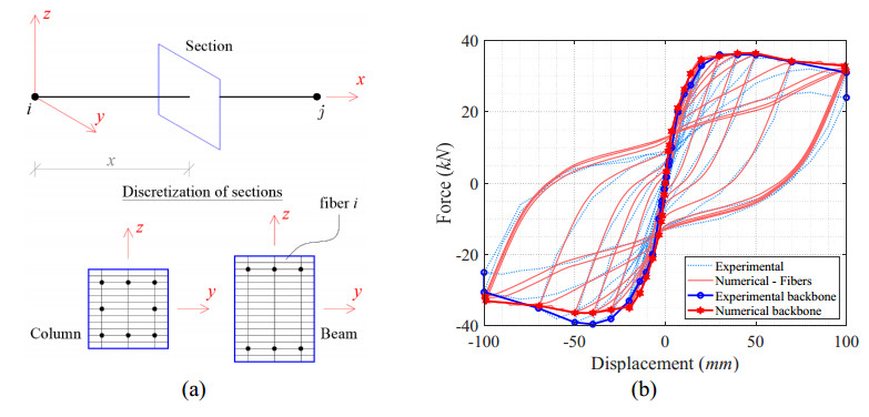
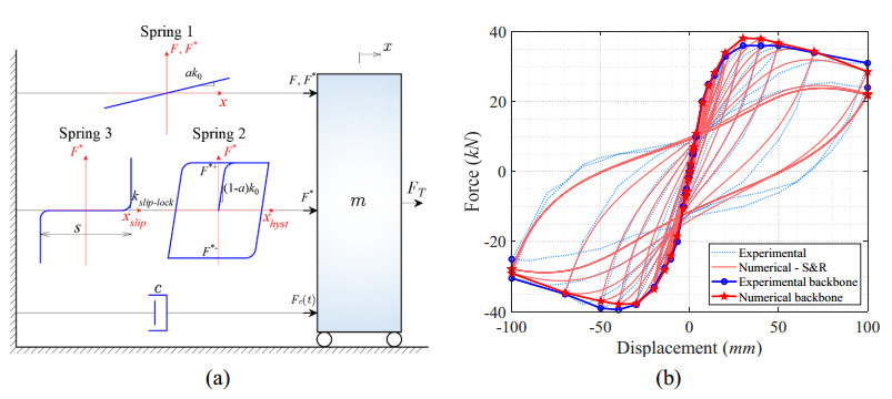
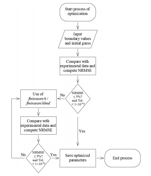
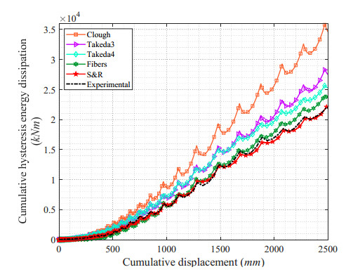
An accurate hysteresis model is fundamental to well capture the non-linearity phenomena occurring in structural and non-structural elements in building structures, that are usually made of reinforced concrete or steel materials. In this sense, this paper aims to numerically estimate through simplified non-linear analyses, the cyclic response of a reinforced concrete frame using different hysteretic models present in the literature. A commercial Finite Element Method package is used to carry out most of the simulations using polygonal hysteretic models and a fiber model, and additionally, a MATLAB script is developed to use a smooth hysteresis model. The experimental data is based on the experiments carried out in the Laboratório Nacional de Engenharia Civil, Portugal. The numerical outcomes are further compared with the experimental result to evaluate the accuracy of the simplified analysis based on the lumped plasticity or plastic hinge method for the reinforced concrete bare frame. Results show that the tetralinear Takeda's model fits closely the experimental hysteresis loops. The fiber model can well capture the hysteresis behavior, though it requires knowledge and expertise on parameter calibration. Sivaselvan and Reinhorn's smooth hysteresis model was able to satisfactorily reproduce the actual non-linear cyclic behavior of the RC frame structure in a global way.
- cyclic response,
- reinforced concrete,
- non-linear analysis,
- hysteresis models,
- optimization
Citation: Pedro Folhento, Manuel Braz-César, Rui Barros. Cyclic response of a reinforced concrete frame: Comparison of experimental results with different hysteretic models[J]. AIMS Materials Science, 2021, 8(6): 917-931. doi: 10.3934/matersci.2021056

Related Papers:

Abstract

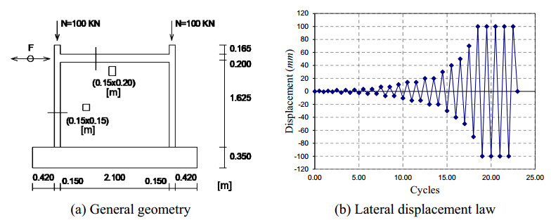
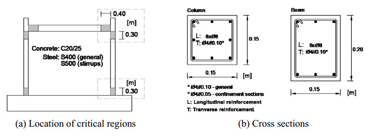
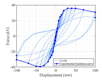
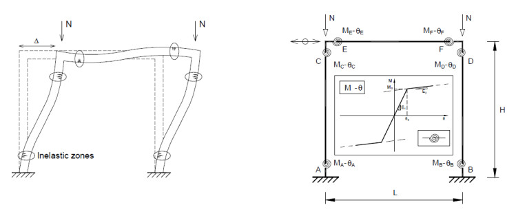
An accurate hysteresis model is fundamental to well capture the non-linearity phenomena occurring in structural and non-structural elements in building structures, that are usually made of reinforced concrete or steel materials. In this sense, this paper aims to numerically estimate through simplified non-linear analyses, the cyclic response of a reinforced concrete frame using different hysteretic models present in the literature. A commercial Finite Element Method package is used to carry out most of the simulations using polygonal hysteretic models and a fiber model, and additionally, a MATLAB script is developed to use a smooth hysteresis model. The experimental data is based on the experiments carried out in the Laboratório Nacional de Engenharia Civil, Portugal. The numerical outcomes are further compared with the experimental result to evaluate the accuracy of the simplified analysis based on the lumped plasticity or plastic hinge method for the reinforced concrete bare frame. Results show that the tetralinear Takeda's model fits closely the experimental hysteresis loops. The fiber model can well capture the hysteresis behavior, though it requires knowledge and expertise on parameter calibration. Sivaselvan and Reinhorn's smooth hysteresis model was able to satisfactorily reproduce the actual non-linear cyclic behavior of the RC frame structure in a global way.

References

[1]	Belleri A, Brunesi E, Nascimbene R, et al. (2015) Seismic performance of precast industrial facilities following major earthquakes in the Italian territory. J Perform Constru Fac 29: 04014135. doi: 10.1061/(ASCE)CF.1943-5509.0000617
[2]	Perrone D, Calvi P, Nascimbene R, et al. (2019) Seismic performance of non-structural elements during the 2016 central Italy earthquake. B Earthq Eng 17: 5655–5677. doi: 10.1007/s10518-018-0361-5
[3]	Brunesi E, Peloso S, Pinho R, et al. (2018) Cyclic testing of a full-scale two-storey reinforced precast concrete wall-slab-wall structure. B Earthq Eng 16: 5309–5339. doi: 10.1007/s10518-018-0359-z
[4]	Bianchi F, Nascimbene R, Pavese A (2017) Experimental vs. numerical aimulations: Seismic response of a half scale three-storey infilled RC building strengthened using FRP retrofit. TOCEJ 11: 1158–1169.
[5]	Nascimbene R (2015) Numerical model of a reinforced concrete building: Earthquake analysis and experimental validation. Period Polytech-Civ 59: 521–530. doi: 10.3311/PPci.8247
[6]	Rahnavard R, Rebelo C, Hélder C, et al. (2020) Numerical investigation of the cyclic performance of reinforced concrete frames equipped with a combination of a rubber core and a U-shaped metallic damper. Eng Struct 225: 111307. doi: 10.1016/j.engstruct.2020.111307
[7]	Visintin A (1994) Differential Models of Hysteresis, Germany: Springer-Verlag.
[8]	Sivaselvan M, Reinhorn A (2000) Hysteretic models for deteriorating inelastic structures. J Eng Mech 126: 633–640. doi: 10.1061/(ASCE)0733-9399(2000)126:6(633)
[9]	Pires F (1990) Influência das paredes de alvenaria no comportamento de estruturas reticuladas de betão armado sujeitas a acções horizontais [PhD Thesis]. LNEC, Lisboa.
[10]	Braz-César M, Oliveira D, Barros R (2008) Comparison of cyclic response of reinforced concrete infilled frames with experimental results. The 14th World Conference on Earthquake Engineering, Beijing, China.
[11]	Fardis M, Panagiotakos T (1997) Seismic design and response of bare and masonry-infilled reinforced concrete buildings. Part Ⅰ: Bare structures. J Earthq Eng 1: 219–256.
[12]	Paulay T, Priestley MJN (1992) Seismic Design of Reinforced Concrete and Masonry Buildings, New York: John Wiley & Sons. doi: 10.1002/9780470172841
[13]	Clough RW (1966) Effects of stiffness degradation on earthquake ductility requirement. UCB/SESM 1966/16, University of California, Berkeley, USA.
[14]	Takeda T, Sozen MA, Nielsen NN (1971) Reinforced concrete response to simulated earthquakes. OHBAYASHI-GUMI Technical Research Report 5, Tokyo, Japan.
[15]	Midas Inc. (2004) Analysis manual: Inelastic time history analysis, Korea.
[16]	Natick, Massachusetts, MATLAB R2019a 9.6.0.1072779, USA: The MathWorks, Inc.
[17]	Deng H, Chang Y, Lau D, et al. (2003) A simplified approach for nonlinear response analysis of composite structural members. International Workshop on Steel and Concrete Composite Constructions NCREE, Taiwan, 207–216.
[18]	Kent D, Park T (1971) Flexural members with confined concrete. J Struct Div 97: 1969–1990. doi: 10.1061/JSDEAG.0002957
[19]	Bouc R (1968) Forced vibration of mechanical systems with hysteresis, In: Rupakhety R, Olafsson S, Bessaon B, Proceedings of the Fourth Conference on Non-linear Oscillation, Prague: Academia.
[20]	Wen Y (1976) Method for random vibration of hysteretic systems. J Eng Mech-ASCE 102: 249–263.
[21]	Wen Y (1980) Equivalent linearization for hysteretic system under random excitation. J Appl Mech 47: 150–154. doi: 10.1115/1.3153594
[22]	D'Errico J (2021) fminsearchbnd, fminsearchcon. Available from: https://www.mathworks.com/matlabcentral/fileexchange/8277-fminsearchbnd-fminsearchcon.

Reader Comments

Your name:*

Email:*
© 2021 the Author(s), licensee AIMS Press. This is an open access article distributed under the terms of the Creative Commons Attribution License (http://creativecommons.org/licenses/by/4.0)