The role of time delays in P53 gene regulatory network stimulated by growth factor

Changyong Dai; Haihong Liu; Fang Yan; Changyong Dai; Haihong Liu; Fang Yan

doi:10.3934/mbe.2020213

Mathematical Biosciences and Engineering

2020, Volume 17, Issue 4: 3794-3835. doi: 10.3934/mbe.2020213

Previous Article Next Article

Research article

The role of time delays in P53 gene regulatory network stimulated by growth factor

1.
Department of Mathematics, Yunnan Normal University, Kunming, 650500, China
2.
Department of Dynamics and Control, Beihang University, Beijing 100191, China

Received: 20 February 2020 Accepted: 21 May 2020 Published: 25 May 2020

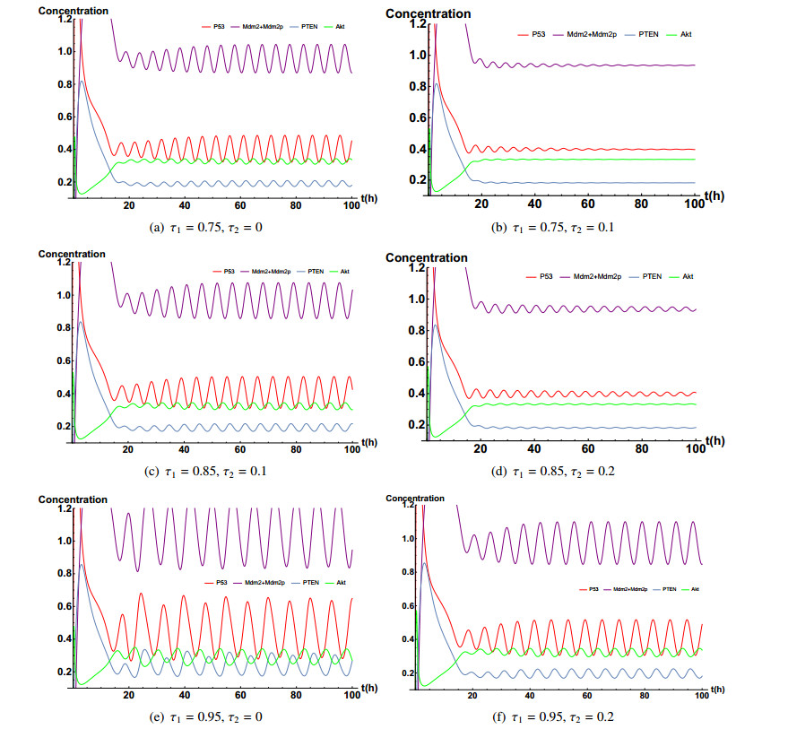
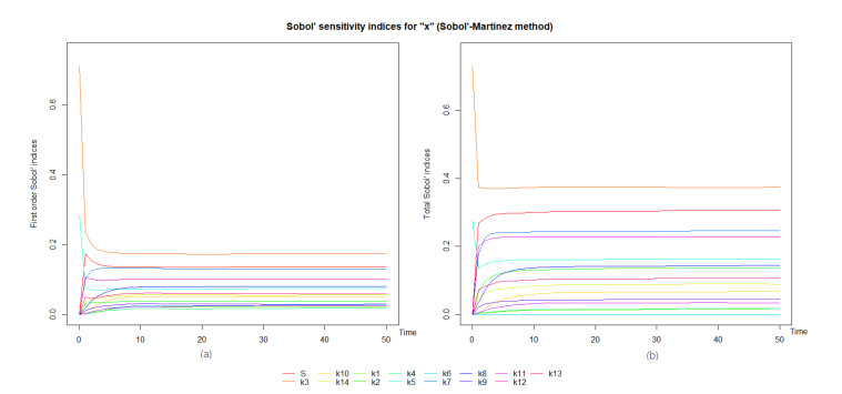
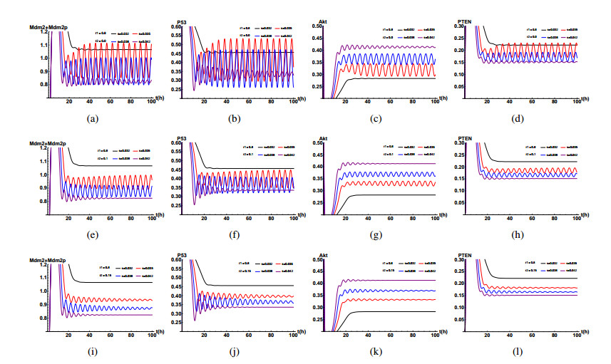
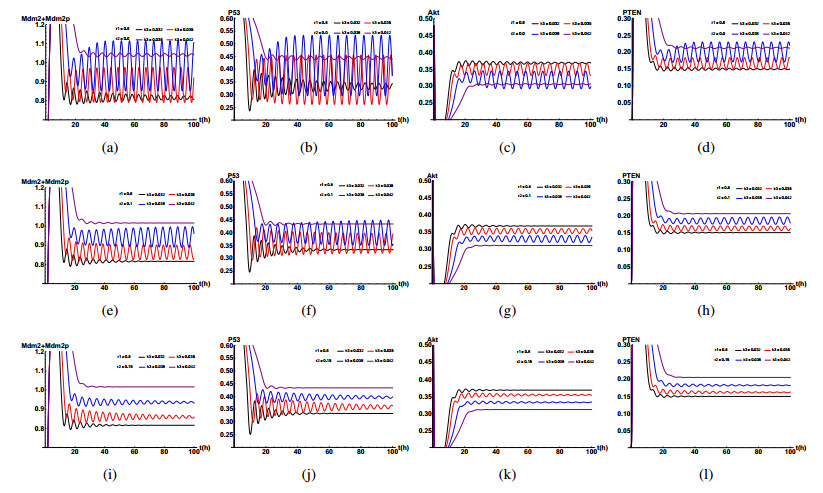
In this paper, a delayed mathematical model for the P53-Mdm2 network is developed. The P53-Mdm2 network we study is triggered by growth factor instead of DNA damage and the amount of DNA damage is regarded as zero. We study the influences of time delays, growth factor and other important chemical reaction rates on the dynamic behaviors in the system. It is shown that the time delay is a critical factor and its length determines the period, amplitude and stability of the P53 oscillation. Furthermore, as for some important chemical reaction rates, we also obtain some interesting results through numerical simulation. Especially, S (growth factor), k₃ (rate constant for Mdm2_p dephosphorylation), k₁₀ (basal expression of PTEN) and k₁₄ (Rate constant for PTEN-induced Akt dephosphorylation) could undermine the dynamic behavior of the system in different degree. These findings are expected to understand the mechanisms of action of several carcinogenic and tumor suppressor factors in humans under normal conditions.

Keywords:

Citation: Changyong Dai, Haihong Liu, Fang Yan. The role of time delays in P53 gene regulatory network stimulated by growth factor[J]. Mathematical Biosciences and Engineering, 2020, 17(4): 3794-3835. doi: 10.3934/mbe.2020213

Related Papers:

[1]	Deniz Sevinç . Volatility spillovers among MIST stock markets. Data Science in Finance and Economics, 2022, 2(2): 80-95. doi: 10.3934/DSFE.2022004
[2]	Nurun Najwa Bahari, Hafizah Bahaludin, Munira Ismail, Fatimah Abdul Razak . Network, correlation, and community structure of the financial sector of Bursa Malaysia before, during, and after COVID-19. Data Science in Finance and Economics, 2024, 4(3): 362-387. doi: 10.3934/DSFE.2024016
[3]	Moses Khumalo, Hopolang Mashele, Modisane Seitshiro . Quantification of the stock market value at risk by using FIAPARCH, HYGARCH and FIGARCH models. Data Science in Finance and Economics, 2023, 3(4): 380-400. doi: 10.3934/DSFE.2023022
[4]	Jiamin Cheng, Yuanying Jiang . How can carbon markets drive the development of renewable energy sector? Empirical evidence from China. Data Science in Finance and Economics, 2024, 4(2): 249-269. doi: 10.3934/DSFE.2024010
[5]	Kuo-Shing Chen . Interlinkages between Bitcoin, green financial assets, oil, and emerging stock markets. Data Science in Finance and Economics, 2024, 4(1): 160-187. doi: 10.3934/DSFE.2024006
[6]	Dachen Sheng, Opale Guyot . Market power, internal and external monitoring, and firm distress in the Chinese market. Data Science in Finance and Economics, 2024, 4(2): 285-308. doi: 10.3934/DSFE.2024012
[7]	Zimei Huang, Zhenghui Li . What reflects investor sentiment? Empirical evidence from China. Data Science in Finance and Economics, 2021, 1(3): 235-252. doi: 10.3934/DSFE.2021013
[8]	Katleho Makatjane, Ntebogang Moroke . Examining stylized facts and trends of FTSE/JSE TOP40: a parametric and Non-Parametric approach. Data Science in Finance and Economics, 2022, 2(3): 294-320. doi: 10.3934/DSFE.2022015
[9]	Samuel Asante Gyamerah, Collins Abaitey . Modelling and forecasting the volatility of bitcoin futures: the role of distributional assumption in GARCH models. Data Science in Finance and Economics, 2022, 2(3): 321-334. doi: 10.3934/DSFE.2022016
[10]	Nitesha Dwarika . The risk-return relationship in South Africa: tail optimization of the GARCH-M approach. Data Science in Finance and Economics, 2022, 2(4): 391-415. doi: 10.3934/DSFE.2022020

Abstract

1. Introduction

When searching the literature, we noticed that several propositions have been made by several researchers to find kernels that can be used to obtain fractional differential operators. The main reason for this is that, real world problems show signs of processes resembling behaviors of some mathematical functions. Riemann, Liouville, Cauchy and Abel works have led to a fractional calculus with a power law kernel. Their work was later modified by Caputo; this version has been used in many fields of science because of its ability to allow classical initial conditions ^[1]. Prabhakar suggested a different kernel as a product of power-law and the generalized Mittag-Leffler function with three parameters. This version has also attracted the attention of many researchers, studies have been done on theory as well as on applications. Indeed, the two kernels have their specific values, for example, power-law helps only to replicate processes exhibiting power-law behavior, while the product of the power-law and the generalized three-parameters Mittag-Leffler has also its field of application ^[2]. As nature is complex, a new kernel was suggested by Caputo and Fabrizio, a special exponential kernel with Delta Dirac properties. A differential operator that is in fashion nowadays due to its ability to replicate processes following fading memory. Indeed, this kernel brought a new shift into fractional calculus, as the concept of the fractional derivative with a non-singular kernel was introduced ^[3]. A point made by some researcher about the non-fractionality of the kernel led to a new kernel, the generalized Mittag-Leffler function with one parameter. This version was suggested by Atangana and Baleanu, constituting another new step forward in the field of fractional calculus. The operators have been used in several fields of studies with great success ^[4]. In ^[5], the basic theory of fractional differentiation, existence-uniqueness theorems and analytical numerical methods of solution of fractional differential equations are presented. In ^[6], the authors examined Noether's theorems of fractional generalized Birkhoffian systems in terms of classical and combined Caputo derivatives. The development of the time-fractional damage model for hyperelastic body is considered in ^[7]. While looking at nature and its complexities, one can with no doubt conclude that these suggested kernels are not enough to predict all complex behaviors of our universe. On this note, one will proceed to search for a different kernel or modified kernel, or a class of functions that will be used to introduce new differential operators. Sabatier recently presented some variants of kernels that will also open new doors for investigation ^[8]. In addition to these outstanding contributions, several other ideas have been suggested, for example the concept of short memory was suggested and a fractional derivative in the Caputo sense has been defined for different values of fractional orders. The idea is to have a different type of variable-order derivative unlike the well-known version that considers a fractional orders. The idea is initiated to have a different type of variable order derivative unlike the well-known version that considers a fractional-order to be a function of time. This case was suggested by Wu et al. ^[9] and applied in chaos. On the other hand, researchers have noticed that several real-world problems exhibit processes with different behaviors as a function of time and space. A particular case is a passage from deterministic to stochastic, or from power law to exponential decay. It was noted that existing differential operators may not be able to account for these behaviors, thus piecewise differential and integral operators were introduced to deal with problems exhibiting crossover behaviors ^[10]. The main aim of this note is to provide a critical analysis of the possible applications, advantages, and disadvantages of these two concepts.

2. Motivation for piecewise derivatives

We will illustrate the motivation with some examples.

Death body decay in different temperatures. Consider a corpse found in a snowy place, and assume that such body has been found after 20 days. The corpse is taken and brought to the house and kept in a normal temperature for a few days and later put in a mortuary and buried. The main aim here is to replicate the process of decay. The first part will provide a very low decay. The second part will provide a fast decay, the third part will again be a fast process and finally, a slow process. Indeed, slow and fast processes can be characterized by some mathematical functions. The power-law function is

$\begin{equation} t^{-\alpha }. \end{equation}$

(2.1)

The exponential decay function with a Dirac delta property is

$\begin{equation} \frac{1}{1-\alpha }\exp \left[ -\frac{\alpha }{1-\alpha }t\right] . \end{equation}$

(2.2)

However, a crossover from fast to slow decay processes can be modeled using the following Mittag-Leffler function with Delta-Dirac property

$\begin{equation} \frac{1}{1-\alpha }E_{\alpha }\left[ -\frac{\alpha }{1-\alpha }t^{\alpha } \right] . \end{equation}$

(2.3)

The process can be divided into several intervals to capture each behavior. In the first part, one can have

$\begin{equation} _{0}^{C}D_{t}^{\alpha }y\left( t\right) = -\lambda _{1}y\left( t\right) \;{\rm{ if }}\;0 < t\leq T_{1}. \end{equation}$

(2.4)

The second processes can be

$\begin{equation} _{T_{1}}^{CF}D_{t}^{\alpha }y\left( t\right) = -\lambda _{2}y\left( t\right) \;{\rm{ if }}\;T_{1} < t\leq T_{2}. \end{equation}$

(2.5)

The two last parts will be characterized by

$\begin{equation} _{T_{2}}^{ABC}D_{t}^{\alpha }y\left( t\right) = -\lambda _{3}y\left( t\right) \; {\rm{ if }}\;T_{2} < t\leq T. \end{equation}$

(2.6)

Thus the whole process will be a system with the following crossover behaviors

$\begin{equation} \left\{ \begin{array}{c} _{0}^{C}D_{t}^{\alpha }y\left( t\right) = -\lambda _{1}y\left( t\right) \;{\rm{ if }}\;0 < t\leq T_{1}, \\ _{T_{1}}^{CF}D_{t}^{\alpha }y\left( t\right) = -\lambda _{2}y\left( t\right) \;{\rm{ if }}\;T_{1} < t\leq T_{2}, \\ _{T_{2}}^{ABC}D_{t}^{\alpha }y\left( t\right) = -\lambda _{3}y\left( t\right) \;{\rm{ if }}\;T_{2} < t\leq T. \end{array} \right. \end{equation}$

(2.7)

Therefore in general the concept of piecewise derivative has been introduced.

3. Short memory concept

In this section, we present the definitions of both short memory and piecewise differentiation. For the short memory case, the idea has already been discussed; for example a paper published by Deng in 2007 has already discussed the short memory principle ^[11], which has also been called the fixed memory principle and logarithmic memory principle. Wu et al. ^[9] presented the concept of a fractional variable-order derivative where the fractional order changes within an interval. The suggested definition is given below as:

$\begin{equation} \left\{ \begin{array}{c} _{t_{0}}^{C}D_{t}^{\alpha _{0}}y\left( t\right)=f\left( y,t\right) \text{ for }t\in \left[ t_{0},t_{1}\right] , \\ _{t_{1}}^{C}D_{t}^{\alpha _{1}}y\left( t\right)=f\left( y,t\right) \text{ for }t\in \left[ t_{1},t_{2}\right] , \\ _{t_{2}}^{C}D_{t}^{\alpha _{2}}y\left( t\right)=f\left( y,t\right) \text{ for }t\in \left[ t_{2},t_{3}\right] . \end{array} \right. \end{equation}$

(3.1)

Here Caputo power law derivative is used, which is known to have a singularity at the origin for a class of functions. The author did not give explicitly space of the functions as the derivative was defined in general, therefore, if we assume a class of the functions for which $\frac{dy}{dt}$ is continuous then at each $t=t_{i},$ $f\left( y,t\right)$ should be zero.

On the other hand, the piecewise concept is defined as follows.

$1)$ A piecewise derivative of $f$ with classical, power-law and stochastic processes is given by

$\begin{equation} \left\{ \begin{array}{c} Dy\left( t\right) = f\left( t,y\left( t\right) \right) \;{\rm{ if }}\;0 < t \leq t_{1}, \\ _{t_{1}}^{C}D_{t}^{\alpha }y\left( t\right) = f\left( t,y\left( t\right) \right) \;{\rm{ if }}\;t_{1} < t\leq t_{2}, \\ dy\left( t\right) = f\left( t,y\left( t\right) \right) dt+\sigma y\left( t\right) dB\left( t\right)\; {\rm{ if }}\;t_{2} < t \leq t_{3}. \end{array} \right. \end{equation}$

(3.2)

$2)$ A piecewise derivative of $f$ with power, exponential and Mittag-Leffler laws is given as

$\begin{equation} \left\{ \begin{array}{c} _{0}^{C}D_{t}^{\alpha }y\left( t\right) = f\left( t,y\left( t\right) \right) \;{\rm{ if }}\;0 < t \leq t_{1}, \\ _{t_{1}}^{CF}D_{t}^{\alpha }y\left( t\right) = f\left( t,y\left( t\right) \right) \;{\rm{ if }}\;t_{1} < t \leq t_{2}, \\ _{t_{1}}^{ABC}D_{t}^{\alpha }y\left( t\right) = f\left( t,y\left( t\right) \right) \;{\rm{ if }}\;t_{2} < t \leq t_{3}. \end{array} \right. \end{equation}$

(3.3)

Several definitions can be found in ^[10] $.$

In the next section, we will provide a deep analysis of these concepts.The aim of the section is to present advantages and disadvantages of these two independent concepts. We note that

$\begin{eqnarray} _{0}^{C}D_{t}^{\alpha }{\rm{ }}f\left( t\right) & = &\frac{1}{\Gamma \left( 1-\alpha \right) }\int\limits_{0}^{t}\frac{d}{d\tau }f\left( \tau \right) \left( t-\tau \right) ^{-\alpha }d\tau ,{\rm{ \ }} \end{eqnarray}$

(3.4)

$\begin{eqnarray} _{0}^{CF}D_{t}^{\alpha }f\left( t\right) & = &\frac{1}{1-\alpha } \int\limits_{0}^{t}\frac{d}{d\tau }f\left( \tau \right) \exp \left[ -\frac{ \alpha }{1-\alpha }\left( t-\tau \right) \right] d\tau , \end{eqnarray}$

(3.5)

$\begin{eqnarray} _{0}^{ABC}D_{t}^{\alpha }f\left( t\right) & = &\frac{1}{1-\alpha } \int\limits_{0}^{t}\frac{d}{d\tau }f\left( \tau \right) E_{\alpha }\left[ - \frac{\alpha }{1-\alpha }\left( t-\tau \right) ^{\alpha }\right] d\tau . \end{eqnarray}$

(3.6)

4. Analysis and difference

Here, we present a deep analysis that will help the readers to see the difference between the two concepts. Let us start with short memory. A deep look inside the short memory concept defined by gives the following:

$1)$ The short memory principle considers a change in constant variable order; however, it uses a single kernel. Indeed, this can be viewed as variable order where the order is changed within shorter intervals. Nonetheless, it describes some process and in the case of Caputo derivation, this process will only describe a power-law process that is, this process will not have crossover behavior.

$2)$ The concept is unable to capture classical processes because the fractional order should change in each interval.

On a serious note, however, if we have $f\left(t, y\left(t\right) \right) \neq 0, \forall t\in \left[ 0, T\right].$ So at each $t_{j}$

$\begin{equation} \lim\limits_{t\rightarrow t_{j}}{\rm{ }}_{t_{j}}^{C}D_{t}^{\alpha }y\left( t\right) = f\left( t,y\left( t\right) \right) \mid _{t = t_{j}}. \end{equation}$

(4.1)

Since $\frac{dy}{dt}$ is continuous,

$\begin{equation} \lim\limits_{t\rightarrow t_{j}}{\rm{ }}_{t_{j}}^{C}D_{t}^{\alpha }y\left( t\right) = f\left( t_{j},y\left( t_{j}\right) \right) \neq 0. \end{equation}$

(4.2)

However the right hand side produces $f\left( t,y\left( t\right) \right) \neq 0$ , which is a contradiction. It infers that $f\left( t_{j},y\left( t_{j}\right) \right) =0.$ This may be used to explain the process with a renewal force that follows the power-law process. For example, the trajectory of a flea with a constant jump. There are fewest real world problems that present these behaviors. However, due to the power-law singularity the definition suggested by Wu may have some problems at the boundaries. Nonetheless, as a result of using non-singular kernels, the concept of short memory will be well-posed since the conditions at the boundaries will be well controlled and the renewal processes would be well-posed

On the other hand, however, the concept of piecewise was introduced for different purposes. The following example will give light to the situation. We consider evaluating the velocity of water within a geological formation with fractures. We record the velocity as a function of time. The velocity will obviously be low in the rock's matrix; however as the water reaches the fracture, there will be a crossover behavior because the velocity will suddenly increase. The first part of this process follows behaviors resembling a declining process and, later, an almost constant high velocity. Now if one was to withdraw water from such a geological formation and record the water level, one will observe a fading groundwater level in earlier times; then when water is being taken from the fracture, we observe a steady groundwater level. Thus, there is a crossover behavior from the fading process to long range, which can be captured using an exponential function, then the power law. Therefore, the differential operator able to replicate this process is

$\begin{equation} \left\{ \begin{array}{c} _{0}^{C}D_{t}^{\alpha }h\left( r,t\right) = f\left( t,r,h\left( r,t\right) \right) \;{\rm{ if }}\;0 < t\leq T_{1}, \\ _{T_{1}}^{CF}D_{t}^{\alpha }h\left( r,t\right) = f_{1}\left( t,r,h\left( r,t\right) \right) \;{\rm{ if }}\;T_{1} < t\leq T. \end{array} \right. \end{equation}$

(4.3)

Therefore, one can see a clear difference and objectives of both concepts. Piecewise differential operators are thus conceived to capture processes exhibiting different patterns, or crossover behaviors. Here the order does not change within an interval as changing order does not change the process but only the memory with the same pattern, rather, the kernels change to bring into the mathematical formulation the crossover behaviors by each kernel.

For example, using the piecewise derivative the decay equation

$\begin{equation} \left\{ \begin{array}{c} y\prime \left( t\right) = -\lambda y\left( t\right) \;{\rm{ if }}\;0 < t\leq T_{1}, \\ _{T_{1}}^{C}D_{t}^{\alpha }y\left( t\right) = -\lambda y\left( t\right) \;{\rm{ if }}\;T_{1} < t\leq T_{2}, \\ dy\left( t\right) = -\lambda y\left( t\right) dt+\sigma y\left( t\right) dB\left( t\right) \;{\rm{ if }}\;T_{2} < t \leq T \end{array} \right. \end{equation}$

(4.4)

which will lead to decay with crossover behaviors. From $0 < t < T_{1}$ , we shall observe a normal decay process. From $T_{1} < t < T_{2}$ , we shall observe power-law decay or the Mittag-Leffler decay. From $T_{2} < t < T$ , we shall observe decay with randomness. On the other hand, with the short memory

$\begin{equation} \left\{ \begin{array}{c} _{0}^{C}D_{t}^{\alpha _{1}}y\left( t\right) = -\lambda y\left( t\right) \;{\rm{ if }}\;0 < t \leq T_{1}, \\ _{T_{1}}^{C}D_{t}^{\alpha _{2}}y\left( t\right) = -\lambda y\left( t\right) \; {\rm{ if }}\;T_{1} < t \leq T_{2}, \\ _{T_{2}}^{C}D_{t}^{\alpha _{3}}y\left( t\right) = -\lambda y\left( t\right) \;{\rm{ if }}\;T_{2} < t \leq T \end{array} \right. \end{equation}$

(4.5)

which leads only to a power-law process or the Mittag-Leffler process.

5. Application to real world problems

In this section, we shall present clearly the difference between the two concepts by applying them to some problems. We shall start with a simple problem about the decay problem with two intervals.

Example 1. We consider a simple decay model within $\left[ 0, T_{1} \right]$ and $\left[ T_{1}, T_{2}\right].$ In the case of short memory, we have

$\begin{equation} \left\{ \begin{array}{c} _{0}^{C}D_{t}^{\alpha _{1}}y\left( t\right) = -\lambda y\left( t\right) \;{\rm{ if }}\;t\in \left[ 0,T_{1}\right] , \\ _{T_{1}}^{C}D_{t}^{\alpha _{2}}y\left( t\right) = -\lambda y\left( t\right) \;{\rm{ if }}\;t\in \left[ T_{1},T_{2}\right]. \end{array} \right. \end{equation}$

(5.1)

In the case of piecewise, we can consider the following

$\begin{equation} \left\{ \begin{array}{c} \frac{dy\left( t\right) }{dt} = -\lambda y\left( t\right) \;{\rm{ if }}\;t\in \left[ 0,T_{1}\right] , \\ _{T_{1}}^{C}D_{t}^{\alpha }y\left( t\right) = -\lambda y\left( t\right) \;{\rm{ if }}\;t\in \left[ T_{1},T_{2}\right] \end{array} \right. \end{equation}$

(5.2)

$\begin{equation} \left\{ \begin{array}{c} _{0}^{ABC}D_{t}^{\alpha }y\left( t\right) = -\lambda y\left( t\right) \;{\rm{ if }}\;t\in \left[ 0,T_{1}\right] , \\ \frac{dy\left( t\right) }{dt} = -\lambda y\left( t\right) \;{\rm{ if }}\;t\in \left[ T_{1},T_{2}\right] \end{array} \right. \end{equation}$

(5.3)

$\begin{equation} \left\{ \begin{array}{c} _{0}^{CF}D_{t}^{\alpha }y\left( t\right) = -\lambda y\left( t\right) \;{\rm{ if }}\;t\in \left[ 0,T_{1}\right] , \\ _{T_{1}}^{C}D_{t}^{\alpha }y\left( t\right) = -\lambda y\left( t\right) \;{\rm{ if }}\;t\in \left[ T_{1},T_{2}\right]. \end{array} \right. \end{equation}$

(5.4)

Using the Laplace transform on the above system yields in the case of short memory

$\begin{equation} \left\{ \begin{array}{c} y\left( t\right) = y\left( 0\right) E_{\alpha _{1}}\left[ -\lambda t^{\alpha _{1}}\right] \;{\rm{ if }}\;t\in \left[ 0,T_{1}\right] , \\ y\left( t\right) = y\left( T_{1}\right) E_{\alpha _{2}}\left[ -\lambda \left( t-T_{1}\right) ^{\alpha _{2}}\right] \;{\rm{ if }}\;t\in \left[ T_{1},T_{2} \right]. \end{array} \right. \end{equation}$

(5.5)

In the case of piecewise, we have the following solution

$\begin{equation} \left\{ \begin{array}{c} y\left( t\right) = y\left( 0\right) \exp \left[ -\lambda t\right] \;{\rm{ if }}\; t\in \left[ 0,T_{1}\right] , \\ y\left( t\right) = y\left( T_{1}\right) E_{\alpha }\left[ -\lambda \left( t-T_{1}\right) ^{\alpha }\right] \;{\rm{ if }}\;t\in \left[ T_{1},T_{2}\right] \end{array} \right. \end{equation}$

(5.6)

$\begin{equation} \left\{ \begin{array}{c} y\left( t\right) = y\left( 0\right) \;{\rm{ if }}\;t = 0, \\ y\left( t\right) = \frac{y\left( 0\right) }{1+\lambda \left( 1-\alpha \right) }E_{\alpha }\left[ -\frac{\lambda \alpha }{1+\lambda \left( 1-\alpha \right) }t^{\alpha }\right] b\;{\rm{ if }}\;t\in \left] 0,T_{1}\right] , \\ y\left( t\right) = y\left( T_{1}\right) \exp \left[ -\lambda \left( t-T_{1}\right) \right] \;{\rm{ if }}\;t\in \left[ T_{1},T_{2}\right] \end{array} \right. \end{equation}$

(5.7)

$\begin{equation} \left\{ \begin{array}{c} y\left( t\right) = y\left( 0\right) \;{\rm{ if }}\;t = 0, \\ y\left( t\right) = \frac{y\left( 0\right) }{1+\lambda \left( 1-\alpha \right) }\exp \left[ -\frac{\lambda \alpha }{1+\lambda \left( 1-\alpha \right) } t^{\alpha }\right] b\;{\rm{ if }}\;t\in \left] 0,T_{1}\right] , \\ y\left( t\right) = y\left( T_{1}\right) E_{\alpha }\left[ -\lambda \left( t-T_{1}\right) ^{\alpha }\right] \;{\rm{ if }}\;t\in \left[ T_{1},T_{2}\right]. \end{array} \right. \end{equation}$

(5.8)

$T_{1} = 1$ where the crossover occurs and $T_{2} = 2.4$ is the final time. The numerical simulations are presented in Figures 1–4 below.

Figure 1. Decay model with short memory for

$\lambda = 3, \alpha _{1} = 0.9$ and

$\alpha _{2} = 0.6$ .

DownLoad: Full-Size Img PowerPoint

Figure 2. Decay model with piecewise derivative for

$\lambda = 3$ .

DownLoad: Full-Size Img PowerPoint

Figure 3. Decay model with piecewise derivative for

$\lambda = 3$ .

DownLoad: Full-Size Img PowerPoint

Figure 4. Decay model with piecewise derivative for

$\lambda = 3$ .

DownLoad: Full-Size Img PowerPoint

Example 2. We consider the spread of an infectious disease. We consider a Susceptible, Exposed, Infected and Recovered (SEIR) model. It was proven by Atangana and Seda that such a model may not be able to predict waves ^[12]. Thus to introduce waves, in particular two waves, we consider the spread to be in the periods $\left[ 0, T_{1} \right]$ and $\left[ T_{1}, T_{2}\right].$ In the case of short memory, we have

$\begin{eqnarray} \left\{ \begin{array}{c} _{0}^{C}D_{t}^{\alpha }S = \mu N-\mu S-\frac{\beta SI}{N} \\ _{0}^{C}D_{t}^{\alpha }E = \frac{\beta SI}{N}-\left( \mu +a\right) E \\ _{0}^{C}D_{t}^{\alpha }I = aE-\left( \gamma +\mu \right) I \\ _{0}^{C}D_{t}^{\alpha }R = \gamma I-\mu R \end{array} \right. \;{\rm{ if }}\;t &\in &\left[ 0,T_{1}\right] , \\ \left\{ \begin{array}{c} _{T_{1}}^{C}D_{t}^{\beta }S = \mu N-\mu S-\frac{\beta SI}{N} \\ _{T_{1}}^{C}D_{t}^{\beta }E = \frac{\beta SI}{N}-\left( \mu +a\right) E \\ _{T_{1}}^{C}D_{t}^{\beta }I = aE-\left( \gamma +\mu \right) I \\ _{T_{1}}^{C}D_{t}^{\beta }R = \gamma I-\mu R \end{array} \right. \;{\rm{ if }}\;t &\in &\left[ T_{1},T_{2}\right] . \end{eqnarray}$

(5.9)

In the case of piecewise several scenarios can be obtained. So we can have

$\begin{eqnarray} \left\{ \begin{array}{c} \overset{\cdot }{S} = \mu N-\mu S-\frac{\beta SI}{N} \\ \overset{\cdot }{E} = \frac{\beta SI}{N}-\left( \mu +a\right) E \\ \overset{\cdot }{I} = aE-\left( \gamma +\mu \right) I \\ \overset{\cdot }{R} = \gamma I-\mu R \end{array} \right. \;{\rm{ if }}\;t &\in &\left[ 0,T_{1}\right] , \\ \left\{ \begin{array}{c} dS = \left( \mu N-\mu S-\frac{\beta SI}{N}\right) dt+\sigma _{1}SdB_{1}\left( t\right) \\ dE = \left( \frac{\beta SI}{N}-\left( \mu +a\right) E\right) dt+\sigma _{2}EdB_{2}\left( t\right) \\ dI = \left( aE-\left( \gamma +\mu \right) I\right) dt+\sigma _{3}IdB_{3}\left( t\right) \\ dR = \left( \gamma I-\mu R\right) dt+\sigma _{4}RdB_{4}\left( t\right) \end{array} \right. \;{\rm{ if }}\;t &\in &\left[ T_{1},T_{2}\right] \end{eqnarray}$

(5.10)

$\begin{eqnarray} \left\{ \begin{array}{c} dS = \left( \mu N-\mu S-\frac{\beta SI}{N}\right) dt+\sigma _{1}SdB_{1}\left( t\right) \\ dE = \left( \frac{\beta SI}{N}-\left( \mu +a\right) E\right) dt+\sigma _{2}EdB_{2}\left( t\right) \\ dI = \left( aE-\left( \gamma +\mu \right) I\right) dt+\sigma _{3}IdB_{3}\left( t\right) \\ dR = \left( \gamma I-\mu R\right) dt+\sigma _{4}RdB_{4}\left( t\right) \end{array} \right. \;{\rm{ if }}\;t &\in &\left[ 0,T_{1}\right] , \\ \left\{ \begin{array}{c} _{T_{1}}^{C}D_{t}^{\alpha }S = \mu N-\mu S-\frac{\beta SI}{N} \\ _{T_{1}}^{C}D_{t}^{\alpha }E = \frac{\beta SI}{N}-\left( \mu +a\right) E \\ _{T_{1}}^{C}D_{t}^{\alpha }I = aE-\left( \gamma +\mu \right) I \\ _{T_{1}}^{C}D_{t}^{\alpha }R = \gamma I-\mu R \end{array} \right. \;{\rm{ if }}\;t &\in &\left[ T_{1},T_{2}\right] . \end{eqnarray}$

(5.11)

Noting that several more scenarios can be considered, however, we will only consider these two in the case of piecewise. Before proceeding with the analysis of these models, we shall first provide an interpolation of each case in terms of wave behaviors. In the case of short memory, the first and second waves show the non-Gaussian distribution associated to the power-law variables $t^{-\alpha _{1}}$ and $t^{-\alpha _{2}}$ . Therefore, one will observe different long tails for $t^{-\alpha _{1}}$ and $t^{-\alpha _{2}}$ . On the other hand, however, the first considered model shows that the first wave has a normal distribution, while the second wave has random behavior. The second model shows that the first wave has a long tail spread while the second has random behavior.

We now present the numerical solutions of the considered models. We shall consider the numerical scheme suggested by Ghanbari et al. ^[13] for fractional cases. The short memory case can be simplified to

$\begin{equation} \left\{ \begin{array}{c} _{0}^{C}D_{t}^{\alpha }y_{i}\left( t\right) = F_{i}\left( t,y_{i}\left( t\right) \right) \;{\rm{ if }}\;t\in \left[ 0,T_{1}\right] , \\ _{T_{1}}^{C}D_{t}^{\beta }y_{i}\left( t\right) = F_{i}\left( t,y_{i}\left( t\right) \right) \;{\rm{ if }}\;t\in \left[ T_{1},T_{2}\right]. \end{array} \right. \end{equation}$

(5.12)

Applying the Ghanbari method yields

$\begin{equation} \left\{ \begin{array}{c} y_{i}^{n_{1}} = y_{i}\left( 0\right) +h^{\alpha }\left( \begin{array}{c} \widetilde{a}_{n_{1}}^{\left( \alpha \right) }F_{i}\left( t_{0},y_{i}\left( t_{0}\right) \right) \\ +\sum\limits_{k = 2}^{n_{1}}\widetilde{a}_{n_{1}-k}^{\left( \alpha \right) }F_{i}\left( t_{k},y_{i}\left( t_{k}\right) \right) \end{array} \right) \;{\rm{ if }}\;t\in \left[ 0,T_{1}\right] , \\ y_{i}^{n_{2}} = y_{i}\left( T_{1}\right) +h^{\beta }\left( \begin{array}{c} \widetilde{a}_{n_{2}}^{\left( \beta \right) }F_{i}\left( T_{1},y_{i}\left( T_{1}\right) \right) \\ +\sum\limits_{j = n_{1}+2}^{n_{2}}a_{n_{2}-j}^{\left( \beta \right) }F_{i}\left( t_{j},y_{i}\left( t_{j}\right) \right) \end{array} \right) \;{\rm{ if }}\;t\in \left[ T_{1},T_{2}\right] \end{array} \right. \end{equation}$

(5.13)

where

$\begin{eqnarray} \widetilde{a}_{n_{1}}^{\left( \alpha \right) } & = &\frac{\left( n_{1}-1\right) ^{\alpha +1}-n_{1}^{\alpha }\left( n_{1}-\alpha -1\right) }{ \Gamma \left( \alpha +2\right) }, \\ a_{n_{2}}^{\left( \beta \right) } & = &\left\{ \begin{array}{c} \frac{1}{\Gamma \left( \beta +2\right) }\;{\rm{ if }}\;n = 0, \\ \frac{\left( n_{2}-1\right) ^{\beta +1}-2n_{2}^{\beta +1}+\left( n_{2}+1\right) ^{\beta +1}}{\Gamma \left( \beta +2\right) }\;{\rm{ if }}\;n\geq 1. \end{array} \right. \end{eqnarray}$

(5.14)

and

$\begin{eqnarray} \widetilde{a}_{n_{2}}^{\left( \beta \right) } &=&\frac{\left( n_{2}-1\right) ^{\beta +1}-n_{2}^{\beta }\left( n_{2}-\beta -1\right) }{\Gamma \left( \beta +2\right) }, \\ \theta _{k}^{\left( \beta \right) } &=&\frac{\left( k-1\right) ^{\beta +1}-2k^{\beta +1}+\left( k+1\right) ^{\beta +1}}{\Gamma \left( \beta +2\right) }\text{ if }k=n_{1}+1,,..,n_{2}-1. \notag \end{eqnarray}$

(5.15)

In the case of the piecewise first model, we have

$\left\{ \begin{matrix} y_{i}^{{{n}_{1}}}={{y}_{i}}\left( 0 \right)+\sum_{j=2}^{{{n}_{1}}}{\left[ \begin{matrix} \frac{23}{12}{{F}_{i}}\left( {{t}_{j}},{{y}_{i}}\left( {{t}_{j}} \right) \right)\Delta t \\ -\frac{4}{3}{{F}_{i}}\left( {{t}_{j-1}},{{y}_{i}}\left( {{t}_{j-1}} \right) \right)\Delta t \\ +\frac{5}{12}{{F}_{i}}\left( {{t}_{j-2}},{{y}_{i}}\left( {{t}_{j-2}} \right) \right)\Delta t \\ \end{matrix} \right]}\ \text{if}\ t\in \left[ 0,{{T}_{1}} \right], \\ \left\{ \begin{matrix} y_{i}^{{{n}_{2}}}=y\left( {{T}_{1}} \right)+\sum_{j={{n}_{1}}+3}^{{{n}_{2}}}{\left[ \begin{matrix} \frac{23}{12}{{F}_{i}}\left( {{t}_{j}},{{y}_{i}}\left( {{t}_{j}} \right) \right)\Delta t \\ -\frac{4}{3}{{F}_{i}}\left( {{t}_{j-1}},{{y}_{i}}\left( {{t}_{j-1}} \right) \right)\Delta t \\ +\frac{5}{12}{{F}_{i}}\left( {{t}_{j-2}},{{y}_{i}}\left( {{t}_{j-2}} \right) \right)\Delta t \\ \end{matrix} \right]}\ \text{if}\ t\in \left[ {{T}_{1}},{{T}_{2}} \right]. \\ +{{\sigma }_{i}}{{y}_{i}}\left( B_{i}^{{{n}_{2}}+1}-B_{i}^{{{n}_{2}}} \right) \\ \end{matrix} \right. \\ \end{matrix} \right.$

(5.16)

For Case 2, we obtain

$\begin{equation} \left\{ \begin{array}{c} \left\{ \begin{array}{c} y_{i}^{n_{1}} = y_{i}\left( 0\right) +\sum_{j = 2}^{n_{1}}\left[ \begin{array}{c} \frac{23}{12}F_{i}\left( t_{j},y_{i}\left( t_{j}\right) \right) \Delta t \\ -\frac{4}{3}F_{i}\left( t_{j-1},y_{i}\left( t_{j-1}\right) \right) \Delta t \\ +\frac{5}{12}F_{i}\left( t_{j-2},y_{i}\left( t_{j-2}\right) \right) \Delta t \end{array} \right] {\rm{ }} \\ +\sigma _{i}\sum_{j = 1}^{n_{1}}y_{j}\left( B_{i}^{j}-B_{i}^{j-1}\right) \end{array} \right. \;{\rm{ if }}\;t\in \left[ 0,T_{1}\right] , \\ y_{i}^{n_{2}} = y_{i}\left( T_{1}\right) +h^{\alpha }\left( \begin{array}{c} \widetilde{a}_{n_{1}}^{\left( \alpha \right) }F_{i}\left( t_{n_{1}},y_{i}\left( t_{n_{1}}\right) \right) \\ +\sum_{k = 0}^{n_{2}}\widetilde{a}_{n_{1}+k}^{\left( \alpha \right) }F_{i}\left( t_{k},y_{i}\left( t_{k}\right) \right) \end{array} \right) \;{\rm{ if }}\;t\in \left[ T_{1},T_{2}\right]. \end{array} \right. \end{equation}$

(5.17)

The numerical solutions for short memory are depicted in Figure 5 with the following parameters

$\begin{equation} N = 1000,\mu = 0.01,\beta = 0.6,a = 0.2,\gamma = 0.03, \end{equation}$

(5.18)

Figure 5. Numerical solutions of Covid-19 model with short memory for

$\alpha _{1} = 0.95, \alpha _{2} = 0.75$ .

DownLoad: Full-Size Img PowerPoint

and the following initial conditions

$\begin{eqnarray} S\left( 0\right) & = &1000,E\left( 0\right) = 25,I\left( 50\right) = 22,R\left( 50\right) = 5,S\left( 50\right) = 39 \\ E\left( 50\right) & = &67,I\left( 50\right) = 505,R\left( 50\right) = 390 \end{eqnarray}$

(5.19)

The numerical solutions for Cases 1 and 2 are respectively depicted in Figures 6 and 7 with the following parameters

$\begin{equation} N = 1000,\mu = 0.01,\beta = 0.6,a = 0.2,\gamma = 0.03, \end{equation}$

(5.20)

Figure 6. Numerical solutions of Covid-19 model under the conditions of Case 1

$\sigma _{1} = 0.000005, \sigma _{2} = 0.008, \sigma _{3} = 0.0021, \sigma _{4} = 0.009$ and

$\alpha = 0.7$ .

DownLoad: Full-Size Img PowerPoint

Figure 7. Numerical solutions of Covid-19 model under the conditions of Case 2

$\sigma _{1} = 0.17, \sigma _{2} = 0.25, \sigma _{3} = 0.21, \sigma _{4} = 0.19$ and

$\alpha = 0.7$ .

DownLoad: Full-Size Img PowerPoint

and the following initial conditions

$\begin{eqnarray} S\left( 0\right) & = &1000,E\left( 0\right) = 25,I\left( 50\right) = 22,R\left( 50\right) = 5,S\left( 50\right) = 35 \\ E\left( 50\right) & = &44,I\left( 50\right) = 424,R\left( 50\right) = 527,\alpha = 0.7 \end{eqnarray}$

(5.21)

demonstrates the short memory effect, where the first and second parts present different long tails behaviors characterized by $\alpha _{1}$ and $\alpha _{2}$ ; however, both clearly depict the same process which is the power law process. On the other hand, Figures 6 and 7 show the clear effects of the piecewise differential operators; the first part in Figure 6 shows normal distribution, which is characteristic of the classical differential operator, while the second part clearly shows the effect of randomness. The complete model therefore shows crossover behavior from deterministic to stochastic with no steady state. In Figure 6, the process is different. We start with randomness then end up with long tail behaviors as a result of the power law kernel.

Example 3. We now consider a chaotic problem in particular the 8-wing attractor ^[14]. This model has been studied by several researchers ^[15], the model is given as

$\begin{eqnarray} \overset{\cdot }{x} & = &a\left( y-x\right) +f\left( t\right) yz \\ \overset{\cdot }{y} & = &cx+dy-xz \\ \overset{\cdot }{z} & = &-bz+xy \end{eqnarray}$

(5.22)

where the function $f\left(t\right) = M$ $sgn\left(\sin \left(wt\right) \right) +K.$ The constant $w$ is known to be a switch frequency and $M$ and $K$ are constant parameters.

In the case of short memory, we have

$\begin{eqnarray} \left\{ \begin{array}{c} _{0}^{C}D_{t}^{\alpha _{1}}x = a\left( y-x\right) +f\left( t\right) yz \\ _{0}^{C}D_{t}^{\alpha _{1}}y = cx+dy-xz \\ _{0}^{C}D_{t}^{\alpha _{1}}z = -bz+xy \end{array} \right. \;{\rm{ if }}\;t &\in &\left[ 0,T_{1}\right] , \\ \left\{ \begin{array}{c} _{T_{1}}^{C}D_{t}^{\alpha _{2}}x = a\left( y-x\right) +f\left( t\right) yz \\ _{T_{1}}^{C}D_{t}^{\alpha _{2}}y = cx+dy-xz \\ _{T_{1}}^{C}D_{t}^{\alpha _{2}}z = -bz+xy \end{array} \right. \;{\rm{ if }}\;t &\in &\left[ T_{1},T_{2}\right] . \end{eqnarray}$

(5.23)

In the case of piecewise, we can consider three cases. For Case 1, we can write

$\begin{eqnarray} \left\{ \begin{array}{c} _{0}^{ABC}D_{t}^{\alpha }x = a\left( y-x\right) +f\left( t\right) yz \\ _{0}^{ABC}D_{t}^{\alpha }y = cx+dy-xz \\ _{0}^{ABC}D_{t}^{\alpha }z = -bz+xy \end{array} \right. \;{\rm{ if }}\;t &\in &\left[ 0,T_{1}\right] , \\ \left\{ \begin{array}{c} dx = \left( a\left( y-x\right) +f\left( t\right) yz\right) dt+\sigma _{1}xdB_{1}\left( t\right) \\ dy = \left( cx+dy-xz\right) dt+\sigma _{2}ydB_{2}\left( t\right) \\ dz = \left( -bz+xy\right) dt+\sigma _{3}zdB_{3}\left( t\right) \end{array} \right. \;{\rm{ if }}\;t &\in &\left[ T_{1},T_{2}\right] . \end{eqnarray}$

(5.24)

For Case 2, we have

$\begin{eqnarray} \left\{ \begin{array}{c} _{0}^{C}D_{t}^{\alpha }x = a\left( y-x\right) +f\left( t\right) yz \\ _{0}^{C}D_{t}^{\alpha }y = cx+dy-xz \\ _{0}^{C}D_{t}^{\alpha }z = -bz+xy \end{array} \right. \;{\rm{ if }}\;t &\in &\left[ 0,T_{1}\right] , \\ \left\{ \begin{array}{c} dx = \left( a\left( y-x\right) +f\left( t\right) yz\right) dt+\sigma _{1}xdB_{1}\left( t\right) \\ dy = \left( cx+dy-xz\right) dt+\sigma _{2}ydB_{2}\left( t\right) \\ dz = \left( -bz+xy\right) dt+\sigma _{3}zdB_{3}\left( t\right) \end{array} \right. \;{\rm{ if }}\;t &\in &\left[ T_{1},T_{2}\right] . \end{eqnarray}$

(5.25)

For Case 3, we can get

$\begin{eqnarray} \left\{ \begin{array}{c} \overset{\cdot }{x} = a\left( y-x\right) +f\left( t\right) yz \\ \overset{\cdot }{y} = cx+dy-xz \\ \overset{\cdot }{z} = -bz+xy \end{array} \right. \;{\rm{ if }}\;t &\in &\left[ 0,T_{1}\right] , \\ \left\{ \begin{array}{c} dx = \left( a\left( y-x\right) +f\left( t\right) yz\right) dt+\sigma _{1}xdB_{1}\left( t\right) \\ dy = \left( cx+dy-xz\right) dt+\sigma _{2}ydB_{2}\left( t\right) \\ dz = \left( -bz+xy\right) dt+\sigma _{3}zdB_{3}\left( t\right) \end{array} \right. \;{\rm{ if }}\;t &\in &\left[ T_{1},T_{2}\right] . \end{eqnarray}$

(5.26)

We shall now present the numerical solution of each case. In the case of short memory, one can use the numerical method based on Lagrange interpolation ^[16]. We can first simplify the model as follows.

$\begin{equation} \left\{ \begin{array}{c} _{0}^{C}D_{t}^{\alpha _{1}}M_{i}\left( t\right) = \Pi \left( t,M_{i}\left( t\right) \right) \;{\rm{ if }}\;t\in \left[ 0,T_{1}\right] , \\ _{T_{1}}^{C}D_{t}^{\alpha _{2}}M_{i}\left( t\right) = \Pi \left( t,M_{i}\left( t\right) \right) \;{\rm{ if }}\;t\in \left[ T_{1},T_{2}\right] \end{array} \right. {\rm{ }}. \end{equation}$

(5.27)

Thus, applying such method to the above system yields

$\begin{equation} \left\{ \begin{array}{c} M_{i}^{n_{1}} = M_{i}\left( 0\right) +\left[ \begin{array}{c} \frac{\left( \Delta t\right) ^{\alpha _{1}}}{\Gamma \left( \alpha _{1}+2\right) }\sum\limits_{q = 0}^{n_{1}}\Pi \left( t_{q},M_{i}^{q}\right) \\ \times \left[ \begin{array}{c} \left( n_{1}-q+1\right) ^{\alpha _{1}}\left( n_{1}-q+2+\alpha _{1}\right) \\ -\left( n_{1}-q\right) ^{\alpha _{1}}\left( n_{1}-q+2+2\alpha _{1}\right) \end{array} \right] \\ -\frac{\left( \Delta t\right) ^{\alpha _{1}}}{\Gamma \left( \alpha _{1}+2\right) }\sum\limits_{q = 1}^{n_{1}}\Pi \left( t_{q-1},M_{i}^{q-1}\right) \\ \times \left[ \begin{array}{c} \left( n_{1}-q+1\right) ^{\alpha _{1}+1} \\ -\left( n_{1}-q\right) ^{\alpha _{1}}\left( n_{1}-q+1+\alpha _{1}\right) \end{array} \right] \end{array} \right] \;{\rm{ if }}\;t\in \left[ 0,T_{1}\right] , \\ M_{i}^{n_{2}} = M_{i}\left( T_{1}\right) +\left[ \begin{array}{c} \frac{\left( \Delta t\right) ^{\alpha _{2}}}{\Gamma \left( \alpha _{2}+2\right) }\sum\limits_{k = n_{1}+1}^{n_{2}}\Pi \left( t_{k},M_{i}^{k}\right) \\ \times \left[ \begin{array}{c} \left( n_{2}-q+1\right) ^{\alpha _{2}}\left( n_{2}-q+2+\alpha _{2}\right) \\ -\left( n_{2}-q\right) ^{\alpha _{2}}\left( n_{2}-q+2+2\alpha _{2}\right) \end{array} \right] \\ -\frac{\left( \Delta t\right) ^{\alpha _{2}}}{\Gamma \left( \alpha _{2}+2\right) }\sum\limits_{k = n_{1}+2}^{n_{2}}\Pi \left( t_{k-1},M_{i}^{k-1}\right) \\ \times \left[ \begin{array}{c} \left( n_{2}-q+1\right) ^{\alpha _{2}+1} \\ -\left( n_{2}-q\right) ^{\alpha _{2}}\left( n_{2}-q+1+\alpha _{2}\right) \end{array} \right] \end{array} \right] \;{\rm{ if }}\;t\in \left[ T_{1},T_{2}\right] \end{array} \right. {\rm{ }}. \end{equation}$

(5.28)

With the piecewise case, we obtain the following numerical solution by using a scheme based on Newton polynomial interpolation ^[17]. Also, we simplify the model as follows.

$\begin{equation} \left\{ \begin{array}{c} _{0}^{ABC}D_{t}^{\alpha _{1}}M_{i}\left( t\right) = \Pi \left( t,M_{i}\left( t\right) \right) \;{\rm{ if }}\;t\in \left[ 0,T_{1}\right] , \\ dM_{i}\left( t\right) = \Pi \left( t,M_{i}\left( t\right) \right) dt+\sigma _{i}M_{i}dB_{i}\left( t\right) \;{\rm{ if }}\;t\in \left[ T_{1},T_{2}\right] \end{array} \right. {\rm{ }}. \end{equation}$

(5.29)

Then applying this method yields

$\begin{equation} \begin{array}{c} M_{i}^{n_{1}} = M_{i}\left( 0\right) +\frac{1-\alpha }{AB\left( \alpha \right) }\Pi \left( t_{n_{1}},M_{i}^{n_{1}}\right) +\frac{\alpha \left( \Delta t\right) ^{\alpha }}{AB\left( \alpha \right) \Gamma \left( \alpha +1\right) } \sum\limits_{k = 2}^{n_{1}}\Pi \left( t_{k-2},M_{i}^{k-2}\right) \\ \times \left\{ \left( n_{1}-k+1\right) ^{\alpha }-\left( n_{1}-k\right) ^{\alpha }\right\} \\ +\frac{\alpha \left( \Delta t\right) ^{\alpha }}{AB\left( \alpha \right) \Gamma \left( \alpha +2\right) }\sum\limits_{k = 2}^{n_{1}}\left[ \Pi \left( t_{k-1},M_{i}^{k-1}\right) -\Pi \left( t_{k-2},M_{i}^{k-2}\right) \right] \\ \times \left\{ \begin{array}{c} \left( n_{1}-k+1\right) ^{\alpha }\left( n_{1}-k+3+2\alpha \right) \\ -\left( n_{1}-k\right) ^{\alpha }\left( n_{1}-k+3+3\alpha \right) \end{array} \right\} \\ +\frac{\alpha \left( \Delta t\right) ^{\alpha }}{2AB\left( \alpha \right) \Gamma \left( \alpha +3\right) }\sum\limits_{k = 2}^{n_{1}}\left[ \Pi \left( t_{k},M_{i}^{k}\right) -2\Pi \left( t_{k-1},M_{i}^{k-1}\right) +\Pi \left( t_{k-2},M_{i}^{k-2}\right) \right] \\ \times \left\{ \begin{array}{c} \left( n_{1}-k+1\right) ^{\alpha }\left[ \begin{array}{c} 2\left( n_{1}-k\right) ^{2}+\left( 3\alpha +10\right) \left( n_{1}-k\right) \\ +2\alpha ^{2}+9\alpha +12 \end{array} \right] \\ -\left( n_{1}-k\right) ^{\alpha }\left[ \begin{array}{c} 2\left( n_{1}-k\right) ^{2}+\left( 5\alpha +10\right) \left( n_{1}-k\right) \\ +6\alpha ^{2}+18\alpha +12 \end{array} \right] \end{array} \right\} ,0\leq t\leq T_{1} \\ \\ M_{i}^{n_{2}+4} = M_{i}^{n_{2}+3}+\sum\limits_{j_{3} = n_{1}+3}^{n_{3}}\left[ \begin{array}{c} \frac{23}{12}\Pi \left( t_{n_{2}+3},M_{i}^{n_{2}+3}\right) -\frac{4}{3}\Pi \left( t_{n_{2}+2},M_{i}^{n_{2}+2}\right) \\ +\frac{5}{12}\Pi \left( t_{n_{2}+1},M_{i}^{n_{2}+1}\right) \end{array} \right] \Delta t \\ +\sigma _{i}M_{i}^{n_{2}}\left( B_{i}^{n_{2}+1}-B_{i}^{n_{2}+1}\right) ,T_{1}\leq t\leq T_{2} \end{array} \end{equation}$

(5.30)

For Case 2, we again apply the scheme with the Newton polynomial to obtain

$\begin{equation} \left\{ \begin{array}{c} M_{i}^{n_{1}} = M_{i}\left( 0\right) +\frac{\left( \Delta t\right) ^{\alpha }}{ \Gamma \left( \alpha +1\right) }\sum\limits_{k = 2}^{n_{1}}\Pi \left( t_{k-2},M_{i}^{k-2}\right) \\ \times \left\{ \left( n_{1}-k+1\right) ^{\alpha }-\left( n_{1}-k\right) ^{\alpha }\right\} \\ +\frac{\left( \Delta t\right) ^{\alpha }}{\Gamma \left( \alpha +2\right) } \sum\limits_{k = 2}^{n_{1}}\left[ \Pi \left( t_{k-1},M_{i}^{k-1}\right) -\Pi \left( t_{k-2},M_{i}^{k-2}\right) \right] , \\ \times \left\{ \begin{array}{c} \left( n_{1}-k+1\right) ^{\alpha }\left( n_{1}-k+3+2\alpha \right) \\ -\left( n_{1}-k\right) ^{\alpha }\left( n_{1}-k+3+3\alpha \right) \end{array} \right\} \\ +\frac{\left( \Delta t\right) ^{\alpha }}{2\Gamma \left( \alpha +3\right) } \sum\limits_{k = 2}^{n_{1}}\left[ \Pi \left( t_{k},M_{i}^{k}\right) -2\Pi \left( t_{k-1},M_{i}^{k-1}\right) +\Pi \left( t_{k-2},M_{i}^{k-2}\right) \right] \\ \times \left\{ \begin{array}{c} \left( n_{1}-k+1\right) ^{\alpha }\left[ \begin{array}{c} 2\left( n_{1}-k\right) ^{2}+\left( 3\alpha +10\right) \left( n_{1}-k\right) \\ +2\alpha ^{2}+9\alpha +12 \end{array} \right] \\ -\left( n_{1}-k\right) ^{\alpha }\left[ \begin{array}{c} 2\left( n_{1}-k\right) ^{2}+\left( 5\alpha +10\right) \left( n_{1}-k\right) \\ +6\alpha ^{2}+18\alpha +12 \end{array} \right] \end{array} \right\} ,0\leq t\leq T_{1} \\ \\ M_{i}^{n_{2}+4} = M_{i}^{n_{2}+3}+\sum\limits_{j_{3} = n_{2}+3}^{n_{3}}\left[ \begin{array}{c} \frac{23}{12}\Pi \left( t_{n_{2}+3},M_{i}^{n_{2}+3}\right) -\frac{4}{3}\Pi \left( t_{n_{2}+2},M_{i}^{n_{2}+2}\right) \\ +\frac{5}{12}\Pi \left( t_{n_{2}+1},M_{i}^{n_{2}+1}\right) \end{array} \right] \Delta t \\ +\sigma _{i}M_{i}\left( C_{n_{2}}\right) \left( B_{i}^{n_{2}+1}-B_{i}^{n_{2}+1}\right) ,T_{1}\leq t\leq T_{2} \end{array} \right. \end{equation}$

(5.31)

where $C_{n_{2}}\in \left[ t_{n_{2}+4}, t_{n_{2}+3}\right]$ . For Case 3, we use the simple Adams-Bashforth methods as follows

$\begin{equation} \left\{ \begin{array}{c} M_{i}^{n_{2}+3} = M_{i}^{n_{2}+2}+\left[ \begin{array}{c} \frac{23}{12}\Pi \left( t_{n_{2}+2},M_{i}^{n_{2}+2}\right) -\frac{4}{3}\Pi \left( t_{n_{2}+1},M_{i}^{n_{2}+1}\right) \\ +\frac{5}{12}\Pi \left( t_{n_{2}},M_{i}^{n_{2}}\right) \end{array} \right] \Delta t,0\leq t\leq T_{1} \\ \\ M_{i}^{n_{2}+4} = M_{i}^{n_{2}+3}+\left[ \begin{array}{c} \frac{23}{12}\Pi \left( t_{n_{2}+3},M_{i}^{n_{2}+3}\right) -\frac{4}{3}\Pi \left( t_{n_{2}+2},M_{i}^{n_{2}+2}\right) \\ +\frac{5}{12}\Pi \left( t_{n_{2}+1},M_{i}^{n_{2}+1}\right) \end{array} \right] \Delta t \\ +\sigma _{i}M_{i}\left( C_{n_{2}}\right) \left( B_{i}^{n_{2}+1}-B_{i}^{n_{2}}\right) ,T_{1}\leq t\leq T_{2} \end{array} \right. \end{equation}$

(5.32)

where $C_{n_{2}}\in \left[ t_{n_{2}+4}, t_{n_{2}+3}\right].$

Numerical solutions are obtained for the following parameters

$\begin{equation} a = 14,b = 43,c = -1,d = 16,M = 9,K = 10,w = \frac{2\pi }{50}. \end{equation}$

(5.33)

The numerical solutions for short memory are depicted in for the initial data $x\left(0\right) = 22.3, y\left(0\right) = 4.9$ and $z\left(0\right) = 2.6.$

Figure 8. Numerical solutions for 8-wing attractor with short memory for

$\alpha _{1} = 0.96$ and

$\alpha _{2} = 0.98$ .

DownLoad: Full-Size Img PowerPoint

For piecewise, we consider the following stochastic-deterministic problem with power-law and Mittag-Leffler kernels:

$\begin{eqnarray} \left\{ \begin{array}{c} _{0}^{C}D_{t}^{\alpha }x = a\left( y-x\right) +f\left( t\right) yz+\sigma _{1}xB\prime _{1}\left( t\right) \\ _{0}^{C}D_{t}^{\alpha }y = cx+dy-xz+\sigma _{2}yB\prime _{2}\left( t\right) \\ _{0}^{C}D_{t}^{\alpha }z = -bz+xy+\sigma _{3}zB\prime _{3}\left( t\right) \end{array} \right. \;{\rm{ if }}\;t &\in &\left[ 0,T_{1}\right] , \\ \left\{ \begin{array}{c} _{{{T}_{1}}}^{ABC}D_{t}^{\alpha }x = a\left( y-x\right) +f\left( t\right) yz \\ _{{{T}_{1}}}^{ABC}D_{t}^{\alpha }y = cx+dy-xz \\ _{{{T}_{1}}}^{ABC}D_{t}^{\alpha }z = -bz+xy \end{array} \right. \;{\rm{ if }}\;t &\in &\left[ T_{1},T_{2}\right] \end{eqnarray}$

(5.34)

with the stochastic constants

$\begin{equation} \sigma _{1} = 0.031;\sigma _{2} = 0.035;\sigma _{3} = 0.032. \end{equation}$

(5.35)

The numerical simulation for such a problem can be performed as illustrated in Figure 9 by using the same initial data and parameters.

Figure 9. Stochastic-deterministic 8-wing attractor with piecewise derivative for

$\alpha = 0.99$ .

DownLoad: Full-Size Img PowerPoint

For piecewise, we consider the following stochastic-deterministic problem with power-law and Mittag-Leffler kernels:

$\begin{eqnarray} \left\{ \begin{array}{c} _{0}^{ABC}D_{t}^{\alpha }x = a\left( y-x\right) +f\left( t\right) yz+\sigma _{1}xB\prime _{1}\left( t\right) \\ _{0}^{ABC}D_{t}^{\alpha }y = cx+dy-xz+\sigma _{2}yB\prime _{2}\left( t\right) \\ _{0}^{ABC}D_{t}^{\alpha }z = -bz+xy+\sigma _{3}zB\prime _{3}\left( t\right) \end{array} \right. \;{\rm{ if }}\;t &\in &\left[ 0,T_{1}\right] , \\ \left\{ \begin{array}{c} _{{{T}_{1}}}^{C}D_{t}^{\alpha }x = a\left( y-x\right) +f\left( t\right) yz \\ _{{{T}_{1}}}^{C}D_{t}^{\alpha }y = cx+dy-xz \\ _{{{T}_{1}}}^{C}D_{t}^{\alpha }z = -bz+xy \end{array} \right. \;{\rm{ if }}\;t &\in &\left[ T_{1},T_{2}\right] \end{eqnarray}$

(5.36)

with the following stochastic constants

$\begin{equation} \sigma _{1} = 0.031;\sigma _{2} = 0.035;\sigma _{3} = 0.032. \end{equation}$

(5.37)

The numerical simulation for such a problem can be performed as shown in Figure 10 by using the same initial data and parameters.

Figure 10. Stochastic-deterministic 8-wing attractor with piecewise derivative for

$\alpha = 0.94$ .

DownLoad: Full-Size Img PowerPoint

Also, we consider the following deterministic-stochastic problem with power-law and Mittag-Leffler kernels:

$\begin{eqnarray} \left\{ \begin{array}{c} _{0}^{C}D_{t}^{\alpha }x = a\left( y-x\right) +f\left( t\right) yz \\ _{0}^{C}D_{t}^{\alpha }y = cx+dy-xz \\ _{0}^{C}D_{t}^{\alpha }z = -bz+xy \end{array} \right. \;{\rm{ if }}\;t &\in &\left[ 0,T_{1}\right] , \\ \left\{ \begin{array}{c} _{{{T}_{1}}}^{ABC}D_{t}^{\alpha }x = a\left( y-x\right) +f\left( t\right) yz+\sigma _{1}xB\prime _{1}\left( t\right) \\ _{{{T}_{1}}}^{ABC}D_{t}^{\alpha }y = cx+dy-xz+\sigma _{2}yB\prime _{2}\left( t\right) \\ _{{{T}_{1}}}^{ABC}D_{t}^{\alpha }z = -bz+xy+\sigma _{3}zB\prime _{3}\left( t\right) \end{array} \right. \;{\rm{ if }}\;t &\in &\left[ T_{1},T_{2}\right] \end{eqnarray}$

(5.38)

with the following stochastic constants:

$\begin{equation} \sigma _{1} = 0.02;\sigma _{2} = 0.012;\sigma _{3} = 0.021. \end{equation}$

(5.39)

The numerical solutions for the above problem can be depicted as shown in Figure 11 using same initial data and parameters.

Figure 11. Deterministic-stochastic 8-wing attractor with piecewise derivative for

$\alpha = 0.99$ .

DownLoad: Full-Size Img PowerPoint

Figure 7 shows the results obtained by applying the power-law short memory concept. To show the difference within the interval, we have opted to consider the first part of the interval to be in blue and the second to be in red. However, a quick look at the results shows clearly the effect of a power law, no great change from one interval to another is observed since both depict long-tail behaviors as results of the power-law kernel. In this case, there is no crossover behavior, just a repetition of different long tail behaviors. On the other hand, in Figures 8 and 9, there is a clear change in patterns where the first patterns show deterministic behaviors in particular, long-tails due to power law in Figure 8, and the second part shows randomness, there is, therefore, a clear crossover from power law to randomness. While, in Figure 9, we have two crossovers, the first is due to the Mittag-Leffler kernel that shows a change from stretched exponential to power law and the second is stochastic.

Also, we consider deterministic-stochastic problem with power-law and Mittag-Leffler kernel

$\begin{eqnarray} \left\{ \begin{array}{c} _{0}^{ABC}D_{t}^{\alpha }x = a\left( y-x\right) +f\left( t\right) yz \\ _{0}^{ABC}D_{t}^{\alpha }y = cx+dy-xz \\ _{0}^{ABC}D_{t}^{\alpha }z = -bz+xy \end{array} \right. \;{\rm{ if }}\;t &\in &\left[ 0,T_{1}\right] , \\ \left\{ \begin{array}{c} _{{{T}_{1}}}^{C}D_{t}^{\alpha }x = a\left( y-x\right) +f\left( t\right) yz+\sigma _{1}xB\prime _{1}\left( t\right) \\ _{{{T}_{1}}}^{C}D_{t}^{\alpha }y = cx+dy-xz+\sigma _{2}yB\prime _{2}\left( t\right) \\ _{{{T}_{1}}}^{C}D_{t}^{\alpha }z = -bz+xy+\sigma _{3}zB\prime _{3}\left( t\right) \end{array} \right. \;{\rm{ if }}\;t &\in &\left[ T_{1},T_{2}\right] \end{eqnarray}$

(5.40)

with the following stochastic constants:

$\begin{equation} \sigma _{1} = 0.02;\sigma _{2} = 0.012;\sigma _{3} = 0.021. \end{equation}$

(5.41)

The numerical solutions for the above problem can be depicted as shown in Figure 12 by using the same initial data and parameters.

Figure 12. Deterministic-stochastic 8-Wing attractor with piecewise derivative for

$\alpha = 0.9$ .

DownLoad: Full-Size Img PowerPoint

6. Conclusions

In the last decades, researchers have devoted their attention to better understanding complex realworld problems even on a small scale. They have therefore developed several methods, different differential, and integral operators. To understand the process by which different long tails occur in different intervals, the concept of short memory was introduced. This concept defines power-law derivatives in different intervals and each interval has its own order. This order accounts for the long tail associated with that interval. However, the process is scale-invariant in terms of patterns. On the other hand, because there are many real-world problems that exhibit passages from one process to another, for example, a passage from power law to randomness, the concept of piecewise was introduced. In this work, a detailed analysis was given to show their different fields of applications and show also, when short memory and piecewise concepts can be applied. This paper thus helps researchers to identify what problem is suitable for short memory and piecewise.

Conflict of interest

The authors declare there is no conflict of interest.

References

[1]	D. W. Meek, Tumour suppression by P53: A role for the DNA damage response, Nat. Rev. Cancer, 9 (2009), 714-723. doi: 10.1038/nrc2716
[2]	V. Rotter, p53, a transformation-related cellular-encoded protein, can be used as a biochemical marker for the detection of primary mouse tumor cells, P Natl. Acad. Sci. USA, 80 (1983), 2613-2617. doi: 10.1073/pnas.80.9.2613
[3]	F. Mantovani, L. Collavin, G. Del Sal, Mutant p53 as a guardian of the cancer cell, Cell Death Differ., 26 (2019), 199-212. doi: 10.1038/s41418-018-0246-9
[4]	J. Bartek, J. Bartkova, B. Vojtesek, Z. Staskova, J. Lukas, A. Rejthar, et al., Aberrant expression of thep53 oncoprotein is a common feature of a wide spectrum of human malignancies, Oncogene, 6 (1991), 1699-1703.
[5]	R. Iggo, J. Bartek, D. Lane, K. Gatter, A. L. Harris, J. Bartek, Increased expression of mutant forms of p53 oncogene in primary lung cancer, Lancet, 335 (1990), 675-679. doi: 10.1016/0140-6736(90)90801-B
[6]	A. J. Levine, P53, the cellular gatekeeper for growth and division, Cell, 88 (1997), 323-331. doi: 10.1016/S0092-8674(00)81871-1
[7]	J. E. Purvis, K. W. Karhohs, C. Mock, E. Batchelor, A. Loewer, G. Lahav, P53 dynamics control cell fate, Science, 336 (2012), 1440-1444. doi: 10.1126/science.1218351
[8]	K. H. Vousden, X. Lu, Live or let die: The cell's response to P53, Nat. Rev. Cancer, 2 (2002), 594-604. doi: 10.1038/nrc864
[9]	B. Vogelstein, D. Lane, A. Levine, Surfing the P53 network, Nature, 408 (2000), 307-310. doi: 10.1038/35042675
[10]	J. D. Oliner, K. W. Kinzler, P. S. Meltzer, D. L. George, B. Vogelstein, Amplification of a gene encoding a P53-associated protein in human sarcomas, Nature, 358 (1992), 80-83. doi: 10.1038/358080a0
[11]	M. H. G. Kubbutat, S. N. Jones, K. H. Vousden, Regulation of P53 stability by Mdm2, Nature, 387 (1997), 299-303. doi: 10.1038/42342-c1
[12]	J. H. Park, S. W. Yang, J. M. Park, S. H. Ka, J. Kim, Y. Kong, et al., Positive feedback regulation of P53 transactivity by DNA damage-induced ISG15 modification, Nat. Commun., 7 (2016), 12513. doi: 10.1038/ncomms12513
[13]	K. H. Vousden, D. P. Lane, P53 in health and disease, Nat. Rev. Mol. Cell Biol., 8 (2007), 275-283. doi: 10.1038/nrm2147
[14]	N. D. Lakin, S. P. Jackson, Regulation of P53 in response to DNA damage, Oncogene, 18 (1999), 7644-7655. doi: 10.1038/sj.onc.1203015
[15]	U. M. Moll, O. Petrenko, The MDM2-P53 interaction, Mol. Cancer Res., 1 (2004), 1001-1008.
[16]	Y. Haupt, R. Maya, A. Kazaz, M. Oren, Mdm2 promotes the rapid degradation of P53, Nature, 387 (1997), 296-299. doi: 10.1038/387296a0
[17]	G. Liao, D. Yang, L. Ma, W. Li, L. Hu, L, Zeng, et al., The development of piperidinones as potent MDM2-P53 protein-protein interaction inhibitors for cancer therapy, Eur. J. Med. Chem., 159 (2018), 1-9. doi: 10.1016/j.ejmech.2018.09.044
[18]	D. Cao, T. K. Ng, Y. W. Y. Yip, A. L. Young, C. P. Pang, W. K. Chu, et al., P53 inhibition by MDM2 in human pterygium, Exp. Eye Res., 175 (2018), 142-147. doi: 10.1016/j.exer.2018.06.021
[19]	R. Li, P. D. Sutphin, D. Schwartz, D. Matas, N. Almog, R. Wolkowicz, et al., Mutant p53 protein expression interferes with p53-independent apoptotic pathways, Oncogene, 16 (1998), 3269-3277. doi: 10.1038/sj.onc.1201867
[20]	G. Blandino, A. J Levine, M. Oren, Mutant p53 gain of function: Differential effects of different p53 mutants on resistance of cultured cells to chemotherapy, Oncogene, 18 (1999), 477-485. doi: 10.1038/sj.onc.1202314
[21]	G. Bossi, E. Lapi, S. Strano, C. Rinaldo, G. Blandino, A. Sacchi, Mutant p53 gain of function: Reduction of tumor malignancy of human cancer cell lines through abrogation of mutant p53 expression, Oncogene, 25 (2006), 304-309. doi: 10.1038/sj.onc.1209026
[22]	M. S. Irwin, K. Kondo, M. C. Marin, L. S. Cheng, W. C. Hahn, W. G. Kaelin, Chemosensitivity linked to p73 function, Cancer Cell, 3 (2003), 403-410. doi: 10.1016/S1535-6108(03)00078-3
[23]	R. Maya, R. Segel, U. Alon, A. J. Levine, Generation of oscillations by the P53-Mdm2 feedback loop: A theoretical and experimental study, P Natl. Acad. Sci. USA, 97 (2000), 11250-11255. doi: 10.1073/pnas.210171597
[24]	L. Ma, J. Wagner, J. Rice, W. Hu, A. Levine, G. Stolovitzky, A plausible model for the digital response of P53 to DNA damage, P Natl. Acad. Sci. USA, 102 (2005), 14266-14271. doi: 10.1073/pnas.0501352102
[25]	T. Zhang, P. Brazhnik, J. J. Tyson, Exploring mechanisms of the DNA-damage response: P53 pulses and their possible relevance to apoptosis, Cell Cycle, 6 (2007), 85-94. doi: 10.4161/cc.6.1.3705
[26]	X. P. Zhang, F. Liu, Z. Cheng, W. Wang, Cell fate decision mediated by P53 pulses, P Natl. Acad. Sci. USA., 106 (2009), 12245-12250. doi: 10.1073/pnas.0813088106
[27]	X. P. Zhang, F. Liu, W. Wang, Two-phase dynamics of P53 in the DNA damage response, P Natl. Acad. Sci. USA, 108 (2011), 8990-8995. doi: 10.1073/pnas.1100600108
[28]	T. Sun, W. Yang, J. Liu, P. Shen, Modeling the basal dynamics of P53 system, PLoS ONE, 6 (2011), e27882. doi: 10.1371/journal.pone.0027882
[29]	B. C. Torrico, M. P. d. A. Filho, T. A. Lima, M. D. D. N. Forte, R. C. Sa, F. G. Nogueira, Tuning of a dead-time compensator focusing on industrial processes, Isa Transact., 83 (2018), 189-198. doi: 10.1016/j.isatra.2018.09.003
[30]	T. Zhang, P. Brazhnik, J. J. Tyson, Computational Analysis of Dynamical Responses to the Intrinsic Pathway of Programmed Cell Death, Biophys J., 97 (2009), 415-434. doi: 10.1016/j.bpj.2009.04.053
[31]	K. H. Chong, S. Samarasinghe, D. Kulasiri, J. Zheng, Mathematical modelling of core regulatory mechanism in P53 protein that activates apoptotic switch, J. Theor. Biol., 462 (2019), 134-147. doi: 10.1016/j.jtbi.2018.11.008
[32]	Y. Zhang, Y. Xiong, W. G. Yarbrough, ARF promotes MDM2 degradation and stabilizes P53: ARF-INK4a locus deletion impairs both the Rb and P53 tumor suppression pathways, Cell, 92 (1998), 725-735. doi: 10.1016/S0092-8674(00)81401-4
[33]	E. Shaulian, D. Resnitzky, O. Shifman, G. Blandino, A. Amsterdam, A. Yayon, et al., Induction of Mdm2 and enhancement of cell survival by bFGF, Oncogene, 15 (1997), 2717-2725. doi: 10.1038/sj.onc.1201453
[34]	Y. Ogawara, S. Kishishita, T. Obata, Y. Isazawa, T. Suzuki, K. Tanaka, et al, Akt enhances Mdm2- mediated ubiquitination and degradation of P53, J. Biol. Chem., 277 (2002), 21843-21850. doi: 10.1074/jbc.M109745200
[35]	A. Carnero, C. Blanco-Aparicio, O. Renner, W. Link, The PTEN/PI3K/Akt signalling pathway in cancer, therapeutic implications, Curr. Cancer Drug Tar., 8 (2008), 187-198. doi: 10.2174/156800908784293659
[36]	X. Tian, B. Huang, X. P. Zhang, M. Lu, W. Wang, Modeling the response of a tumor-suppressive network to mitogenic and oncogenic signals, P Natl. Acad. Sci. USA, 114 (2017), 5337-5342. doi: 10.1073/pnas.1702412114
[37]	B. Novak, J. J. Tyson, Design principles of biochemical oscillators, Nat. Rev. Mol. Cell Biol., 9 (2008), 981-991. doi: 10.1038/nrm2530
[38]	J. R. Pomerening, S. Y. Kim, J. E. Ferrell, Systems-level dissection of the cell-cycle oscillator: Bypassing positive feedback produces damped oscillations, Cell, 122 (2005), 565-578. doi: 10.1016/j.cell.2005.06.016
[39]	K. Jonak, M. Kurpas, K. Szoltysek, J. Patryk, A. Abramowicz, K. Puszynski, A novel mathematical model of ATM/P53/NF-kB pathways points to the importance of the DDR switch-off mechanisms, BMC Syst. Biol., 10 (2016), 75. doi: 10.1186/s12918-016-0293-0
[40]	A. Honkela, J. Peltonen, H. Topa, I. Charapitsa, F. Matarese, Genome-wide modeling of transcription kinetics reveals patterns of RNA production delays, P Natl. Acad. Sci. USA, 112 (2015), 13115-13120. doi: 10.1073/pnas.1420404112
[41]	A. Prindle, J. Selimkhanov, H. Li, I. Razinkov, L. S. Tsimring, J. Hasty, Rapid and tunable post-translational coupling of genetic circuits, Nature, 508 (2014), 387-391. doi: 10.1038/nature13238
[42]	H. K. Yalamanchili, B. Yan, M. J. Li, J. Qin, Z. Zhao, F. Y. L. Chin, et al., DDGni: Dynamic delay gene-network inference from high-temporal data using gapped local alignment, Bioinformatics, 30 (2014), 377-383. doi: 10.1093/bioinformatics/btt692
[43]	V. Stambolic, D. Macpherson, D. Sas, Y. Lin, B. Snow, Regulation of PTEN transcription by P53, Mol. Cell, 8 (2001), 317-325. doi: 10.1016/S1097-2765(01)00323-9
[44]	Y. Barak, E. Gottlieb, T. Juven-Gershon, M. Oren, Regulation of mdm2 expression by P53: Alternative promoters produce transcripts with nonidentical translation potential, Gene Dev., 8 (1994), 1739-1749. doi: 10.1101/gad.8.15.1739
[45]	K. B. Wee, B. D. Aguda, Akt versus P53 in a network of oncogenes and tumor suppressor genes regulating cell survival and death, Biophys J., 91 (2006), 857-865. doi: 10.1529/biophysj.105.077693
[46]	D. Qiu, L. Mao, S. Kikuchi, M. Tomita, Sustained MAPK activation is dependent on continual NGF receptor regeneration, Dev. Growth Differ., 46 (2004), 393-403. doi: 10.1111/j.1440-169x.2004.00756.x
[47]	B. N. Kholodenko, Negative feedback and ultrasensitivity can bring about oscillations in the mitogen-activated protein kinase cascades, Eur. J. Biochem., 267 (2000), 1583-1588. doi: 10.1046/j.1432-1327.2000.01197.x
[48]	Y. Zhang, H. Liu, F. Yan, J. Zhou, Oscillatory dynamics of p38 activity with transcriptional and translational time delays, Sci. Rep. 7, (2017), 11495. doi: 10.1038/s41598-017-11149-5
[49]	Y. Harima, Y. Takashima, Y. Ueda, T. Ohtsuka, R. Kageyama, Accelerating the tempo of the segmentation clock by reducing the number of introns in the Hes7 gene, Cell Rep., 3, (2013), 1-7. doi: 10.1016/j.celrep.2012.11.012
[50]	Y. Takashima, T. Ohtsuka, A. Gonzalez, H. Miyachi, R. Kageyama, Intronic delay is essential for oscillatory expression in the segmentation clock, P Natl. Acad. Sci. USA, 108, (2011), 3300-3305.
[51]	J. Lewis, Autoinhibition with transcriptional delay: A simple mechanism for the zebrafish somitogenesis oscillator, Curr. Biol., 13, (2003), 1398-1408. doi: 10.1016/S0960-9822(03)00534-7
[52]	A. Audibert, D. Weil, F. Dautry, In vivo kinetics of mrna splicing and transport in mammalian cells, Mol. Cell Biol., 22, (2002), 6706-6718. doi: 10.1128/MCB.22.19.6706-6718.2002
[53]	J. Fruth, New methods for the sensitivity analysis of black-box functions with an application to sheet metal forming, TU Dortmund University, 2015.
[54]	B. P. Zhou, Y. Liao, W. Xia, Y. Zou, B. Spohn, M.C. Hung, HER-2/neu induces P53 ubiquitination via Akt-mediated MDM2 phosphorylation, Nat. Cell Biol., 3 (2001), 973-982. doi: 10.1038/ncb1101-973
[55]	S. Ruan, J. Wei, On the zeros of transcendental functions with applications to stability of delay differential equations with two delays, Dynam. Cont. Dis. Ser. A, 10 (2003), 863-874.
[56]	B. D. Hassard, N. D. Kazarinoff, Y. H. Wan, Theory and applications of Hopf bifurcation, Cambridge University Press, 1981.

This article has been cited by:

1.	Rodrigo Moreira, Larissa Ferreira Rodrigues Moreira, Flávio de Oliveira Silva, Brazilian Selic Rate Forecasting with Deep Neural Networks, 2024, 0927-7099, 10.1007/s10614-024-10597-2
2.	Michele Bufalo, Claudia Ceci, Giuseppe Orlando, Addressing the financial impact of natural disasters in the era of climate change, 2024, 73, 10629408, 102152, 10.1016/j.najef.2024.102152
3.	Guo-Hui Yang, Si-Qi Ma, Xiao-Dong Bian, Jiang-Cheng Li, Pierluigi Vellucci, The roles of liquidity and delay in financial markets based on an optimal forecasting model, 2023, 18, 1932-6203, e0290869, 10.1371/journal.pone.0290869
4.	Giacomo Ascione, Michele Bufalo, Giuseppe Orlando, Modeling volatility of disaster-affected populations: A non-homogeneous geometric-skew Brownian motion approach, 2024, 130, 10075704, 107761, 10.1016/j.cnsns.2023.107761

Reader Comments

Your name:*

Email:*
© 2020 the Author(s), licensee AIMS Press. This is an open access article distributed under the terms of the Creative Commons Attribution License (http://creativecommons.org/licenses/by/4.0)