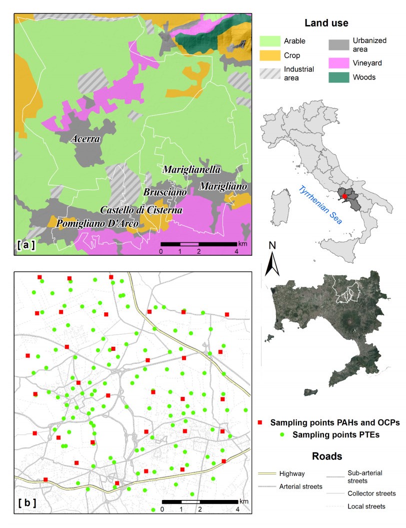
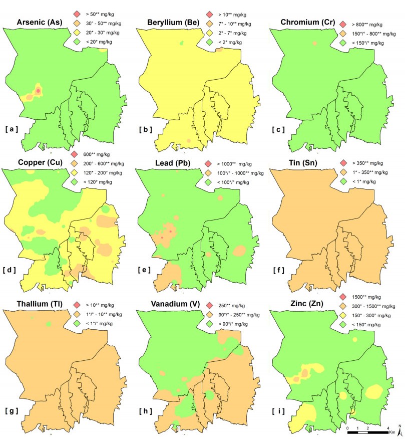
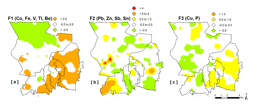
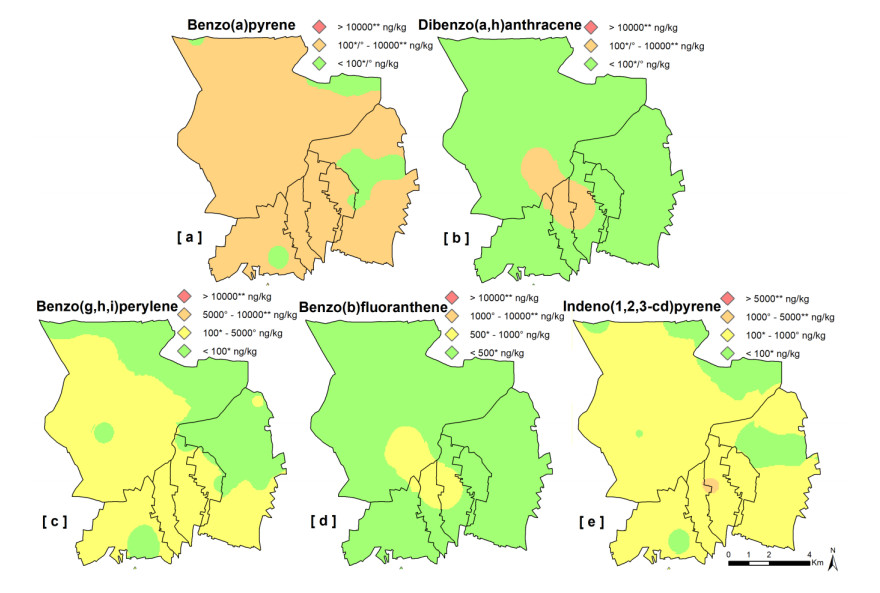
Epidemiological and environmental studies demonstrated that the rate of cancer mortality in the Acerra area, better known as "Triangle of Death", and, more in general, in the Neapolitan metropolitan territory are higher than the regional average values. In the "Triangle of Death" the higher rate of mortality has been mostly related to the presence of toxic wastes illegally buried in agricultural areas which have been contaminating soils and groundwater for decades. Thus, collecting a total of 154 samples over an area of about 100 km2, a detailed study was carried out to assess the geochemical-environmental conditions of soils aiming at defining the environmental hazard proceeding from 15 potentially toxic elements (PTEs), 9 polycyclic aromatic hydrocarbons (PAHs) and 14 organochlorine pesticides (OCPs) related with soil contamination. The study was also targeted at discriminating the contamination sources of these pollutants. Results showed that 9 PTEs, 5 PAHs and 6 OCPs are featured by concentrations higher than the guideline values established by the Italian Environmental laws, especially in the proximities of inhabited centers and industrial areas. The contamination source analysis revealed that, as regards the concentrations of chemical elements, they have a dual origin due to both the natural composition of the soils (Co-Fe-V-Tl-Be) and the pressure exerted on the environment by anthropic activities such as vehicular traffic (Pb-Zn-Sb-Sn) and agricultural practices (Cu-P). As far as organic compounds are concerned, the source of hydrocarbons can be mainly attributed to the combustion of biomass (i.e., grass, wood and coal), while for pesticides, although the use of some of them has been prohibited in Italy since the 1980s, it has been found that they are still widely used by local farmers.
Citation: Stefano Albanese, Annalise Guarino. Assessing contamination sources and environmental hazards for potentially toxic elements and organic compounds in the soils of a heavily anthropized area: the case study of the Acerra plain (Southern Italy)[J]. AIMS Geosciences, 2022, 8(4): 552-578. doi: 10.3934/geosci.2022030
Epidemiological and environmental studies demonstrated that the rate of cancer mortality in the Acerra area, better known as "Triangle of Death", and, more in general, in the Neapolitan metropolitan territory are higher than the regional average values. In the "Triangle of Death" the higher rate of mortality has been mostly related to the presence of toxic wastes illegally buried in agricultural areas which have been contaminating soils and groundwater for decades. Thus, collecting a total of 154 samples over an area of about 100 km2, a detailed study was carried out to assess the geochemical-environmental conditions of soils aiming at defining the environmental hazard proceeding from 15 potentially toxic elements (PTEs), 9 polycyclic aromatic hydrocarbons (PAHs) and 14 organochlorine pesticides (OCPs) related with soil contamination. The study was also targeted at discriminating the contamination sources of these pollutants. Results showed that 9 PTEs, 5 PAHs and 6 OCPs are featured by concentrations higher than the guideline values established by the Italian Environmental laws, especially in the proximities of inhabited centers and industrial areas. The contamination source analysis revealed that, as regards the concentrations of chemical elements, they have a dual origin due to both the natural composition of the soils (Co-Fe-V-Tl-Be) and the pressure exerted on the environment by anthropic activities such as vehicular traffic (Pb-Zn-Sb-Sn) and agricultural practices (Cu-P). As far as organic compounds are concerned, the source of hydrocarbons can be mainly attributed to the combustion of biomass (i.e., grass, wood and coal), while for pesticides, although the use of some of them has been prohibited in Italy since the 1980s, it has been found that they are still widely used by local farmers.

| [1] | Albanese S, Breward N (2011) Sources of Anthropogenic Contaminants in the Urban Environment, In: Johnson CC, Author, Mapping the chemical environment of urban areas, Wiley, 116–127. |
| [2] |
Albanese S, Cicchella D (2012) Legacy problems in urban geochemistry. Elements 8: 423–428. https://doi.org/10.2113/gselements.8.6.423 doi: 10.2113/gselements.8.6.423

|
| [3] | WHO, Air quality guidelines for particulate matter, ozone, nitrogen dioxide and sulphur dioxide—Global update 2005—Summary of risk assessment. World Health Organization, Geneva, Switzerland, 2006. |
| [4] | Ali H, Khan E, Ilahi I (2019) Environmental chemistry andecotoxicology of hazardous heavy metals: environmental per-sistence, toxicity, and bioaccumulation. J Chem, 1–14. |
| [5] | Liu J, Goyer RA, Waalkes MP (2007) Toxic effects of metals, In: Klaassen CD, Author, Casarett and Doull's Toxicology: The Basic Science of Poisons, 7 Eds., New York: McGraw-Hill Professional, 931–980. |
| [6] |
Antoniadis V, Shaheen SM, Levizou E, et al. (2019) A critical prospective analysis of the potential toxicity of trace element regulation limits in soils worldwide: Are they protective concerning health risk assessment?—A review. Environ Int 127: 819–847. https://doi.org/10.1016/j.envint.2019.03.039 doi: 10.1016/j.envint.2019.03.039
|
| [7] | Fengpeng H, Zhihuan Z, Yunyang W, et al. (2009) Polycyclic aromatic hydrocarbons in soils of Beijing and Tianjin region: Vertical distribution, correlation with TOC and transport mechanism. J Environ Sci 21: 675–685. |
| [8] |
Manoli E, Kouras A, Samara C (2004) Profile analysis of ambient and source emitted particle-bound polycyclic aromatic hydrocarbons from three sites in northern Greece. Chemosphere 56: 867–878. https://doi.org/10.1016/j.chemosphere.2004.03.013 doi: 10.1016/j.chemosphere.2004.03.013
|
| [9] | ATSDR, Toxicity of Polycyclic Aromatic Hydrocarbons (PAHs). Agency for Toxic Substances and Disease Registry (ATSDR), Atlanta GA, 2009. Available from: https://www.atsdr.cdc.gov/csem/pah/docs/pah.pdf. |
| [10] | Eisler R (2000) Handbook of Chemical Risk Assessment: Health Hazards to Humans, Plants and Animals, Boca Raton: Lewis Publishers. |
| [11] | USEPA, Ambient water quality criteria for polynuclear aromatic hydrocarbons. United States Environmental Protection Agency (USEPA), Washington, DC, 1980. Available from: https://www.epa.gov/sites/default/files/2019-03/documents/ambient-wqc-pah-1980.pdf. |
| [12] | Sparling DW (2016) Ecotoxicology Essentials. Polycyclic Aromatic Hydrocarbons. 1 Eds., Amsterdam: Elsevier, 193–221. |
| [13] | Schaefer C, Peters P, Miller RK (2015) Drugs During Pregnancy and Lactation. 3 Eds., Amsterdam: Elsevier. |
| [14] | ISPRA, Impatto sugli ecosistemi e sugli esseri viventi delle sostanze sintetiche utilizzate nella profilassi anti-zanzara. Istituto Superiore per la Protezione e la Ricerca Ambientale (ISPRA), 2015. Available from: https://www.isprambiente.gov.it/files/pubblicazioni/quaderni/ambiente-societa/Quad_AS_10_15_ProfilassiAntiZanzare.pdf. |
| [15] |
Lushchak VI, Matviishyn TM, Husak VV, et al. (2018) Pesticide toxicity: A mechanistic approach. EXCLI J 1: 1101–1136. https://doi.org/10.17179/excli2018-1710 doi: 10.17179/excli2018-1710
|
| [16] |
Balmer JE, Morris AD, Hung H, et al. (2019) Levels and trends of current-use pesticides (CUPs) in the arctic: an updated review, 2010–2018. Emerg Contam 5: 70–88. https://doi.org/10.1016/j.emcon.2019.02.002 doi: 10.1016/j.emcon.2019.02.002
|
| [17] | Sparling DW (2016) Ecotoxicology Essentials. Organochlorine Pesticides. 1 Eds., Amsterdam: Elsevier, 69–107. |
| [18] |
Kim KH, Kabir E, Jahan SA (2017) Exposure to pesticides and the associated human health effects. Sci Total Environ 575: 525–535. https://doi.org/10.1016/j.scitotenv.2016.09.009 doi: 10.1016/j.scitotenv.2016.09.009
|
| [19] | Stockholm Convention on Persistent Organic Pollutants, Worldwide found, Stockholm convention "new POPs": screening additional POPs candidates, 2005. Available from: http://chm.pops.int/TheConvention/ThePOPs/TheNewPOPs/tabid/2511/Default.aspx. |
| [20] | Stockholm Convention on Persistent Organic Pollutants, 2011. Available from: http://chm.pops.int/. |
| [21] | IARC, Monographs evaluate DDT, lindane, and 2, 4-D. Press Release Number 236. International Agency for Research on Cancer (IARC), 2015. Available from: https://www.iarc.who.int/wp-content/uploads/2018/07/pr236_E.pdf. |
| [22] |
Senior K, Mazza A (2004) Italian "Triangle of death" linked to waste crisis. Lancet Oncol 5: 525–527. https://doi.org/10.1016/s1470-2045(04)01561-x doi: 10.1016/s1470-2045(04)01561-x
|
| [23] | Flora A (2015) La Terra dei Fuochi: ambiente e politica industriale nel Mezzogiorno. Riv Econ Del Mezzogiorno Trimest Svimez 1–2: 89–122. |
| [24] |
Albanese S, De Vivo B, Lima A, et al. (2007) Geochemical background and baseline values of toxic elements in stream sediments of Campania region (Italy). J Geochem Explor 93: 21–34. https://doi.org/10.1016/j.gexplo.2006.07.006 doi: 10.1016/j.gexplo.2006.07.006
|
| [25] | Albanese S, De Luca ML, De Vivo B, et al. (2008) Relationships between heavy metals distribution and cancer mortality rates in the Campania Region, Italy, In: De Vivo B, Belkin HE, Lima A, Authors, Environmental Geochemistry: Site Characterization, Data Analysis and Case Histories, Amsterdam: Elsevier, 391–404. |
| [26] | Albanese S, Cicchella D, De Vivo B, et al. (2011) Advancements in urban geochemical mapping of the Naples metropolitan area: color composite maps and results from an urban brownfield site, In: Johnson CC, Demetriades A, Locutura J, Authors, Mapping The Chemical Environment of Urban Areas, UK: John Wiley Publisher, 410–423. |
| [27] |
Bove M, Ayuso RA, De Vivo B, et al. (2011) Geochemical and isotopic study of soils and waters from an Italian contaminated site: Agro Aversano (Campania). J Geochem Explor 109: 38–50. https://doi.org/10.1016/j.gexplo.2010.09.013 doi: 10.1016/j.gexplo.2010.09.013
|
| [28] |
Catani V, Zuzolo D, Esposito L, et al. (2020) A New Approach for Aquifer Vulnerability Assessment: the Case Study of Campania Plain. Water Resour Manage 34: 819–834. https://doi.org/10.1007/s11269-019-02476-5 doi: 10.1007/s11269-019-02476-5
|
| [29] |
Cicchella D, De Vivo B, Lima A, et al. (2008) Heavy metal pollution and Pb isotopes in urbansoils of Napoli, Italy. Geochem Explor Environ Anal 8: 103–112. https://doi.org/10.1144/1467-7873/07-148 doi: 10.1144/1467-7873/07-148
|
| [30] | De Vivo B, Lima A, Albanese S, et al. (2006) Atlante geochimico-ambientale dei suoli dell'area urbana e della provincia di Napoli, Roma: Aracne Editrice. |
| [31] | De Vivo B, Lima A, Albanese S, et al. (2016) Atlante geochimico-ambientale dei suoli della Campania, Roma: Aracne Editrice. |
| [32] | De Vivo B, Albanese S, Lima A, et al. (2021) Composti Organici Persistenti: Idrocarburi Policiclici Aromatici, Policlorobifenili, Pesticidi, Monitoraggio Geochimico-Ambientale dei suoli della Regione Campania, Roma: Aracne Editrice. |
| [33] | De Vivo B, Cicchella D, Lima A, et al. (2021) Elementi Potenzialmente Tossici e loro Biodisponibilità, Elementi Maggiori e in Traccia; distribuzione in suoli superficiali e profondi, Monitoraggio Geochimico-Ambientale dei suoli della Regione Campania, Roma: Aracne Editrice. |
| [34] | De Vivo B, Cicchella D, Albanese S, et al. (2022) Idrocarburi Policiclici Aromatici (IPA), Policlorobifenili (PCB), Pesticidi (OCP), Eteri di Polibromobifenili (PBDE), Elementi Potenzialmente Tossici (EPT), Monitoraggio geochimico-ambientale della matrice aria della Regione Campania. Il Piano Campania Trasparente, Roma: Aracne Editrice. |
| [35] |
Grezzi G, Ayuso RA, De Vivo B, et al. (2011) Lead isotopes in soils and ground waters as tracers of the impact of human activities on the surface environment: the Domizio-flegreo littoral (Italy) case study. J Geochem Explor 109: 51–58. https://doi.org/10.1016/j.gexplo.2010.09.012 doi: 10.1016/j.gexplo.2010.09.012
|
| [36] | Lima A, Giaccio L, Cicchella D, et al. (2012) Atlante geochimico ambientale del S.I.N-Litorale Domizio flegreo e Agro aversano, Roma: Aracne editrice. |
| [37] |
Minolfi G, Albanese S, Lima A, et al. (2018) Human health risk assessment in Avellino-Salerno metropolitan areas, Campania Region, Italy. J Geochem Explor 195: 97–109. https://doi.org/10.1016/j.gexplo.2017.12.011 doi: 10.1016/j.gexplo.2017.12.011
|
| [38] |
Minolfi G, Petrik A, Albanese S, et al. (2019) The distribution of Pb, Cu and Zn in topsoil of the Campanian Region, Italy. Geochem: Explor Environ Anal 19: 205–215. https://doi.org/10.1144/geochem2017-074 doi: 10.1144/geochem2017-074
|
| [39] |
Petrik A, Albanese S, Lima A, et al. (2018) The spatial pattern of beryllium and its possible origin using compositional data analysis on a high-density topsoil data set from the Campania Region (Italy). Appl Geochem 91: 162–173. https://doi.org/10.1016/j.apgeochem.2018.02.008 doi: 10.1016/j.apgeochem.2018.02.008
|
| [40] |
Petrik A, Thiombane M, Albanese S, et al. (2018) Source patterns of Zn, Pb, Cr and Ni potentially toxic elements (PTEs) through a compositional discrimination analysis: A case study on the Campanian topsoil data. Geoderma 331: 87–99. https://doi.org/10.1016/j.geoderma.2018.06.019 doi: 10.1016/j.geoderma.2018.06.019
|
| [41] |
Petrik A, Albanese S, Lima A, et al. (2018) Spatial pattern recognition of arsenic in topsoil using high-density regional data. Geochem Explor Environ Anal 18: 319–330. https://doi.org/10.1144/geochem2017-060 doi: 10.1144/geochem2017-060
|
| [42] |
Petrik A, Albanese S, Lima A, et al. (2018) Spatial pattern analysis of Ni and its concentrations in topsoils in the Campania region (Italy). J Geochem Explor 195: 130–142. https://doi.org/10.1016/j.gexplo.2017.09.009 doi: 10.1016/j.gexplo.2017.09.009
|
| [43] |
Petrik A, Thiombane M, Lima A, et al. (2018) Soil Contamination Compositional Index: a new approach to quantify contamination demonstrated by assessing compositional source patterns of potentially toxic elements in the Campania Region (Italy). Appl Geochem 96: 264–276. https://doi.org/10.1016/j.apgeochem.2018.07.014 doi: 10.1016/j.apgeochem.2018.07.014
|
| [44] |
Qu C, Albanese S, Chen W, et al. (2016) The status of organochlorine pesticide contamination in the soils of the Campanian Plain, southern Italy, and correlations with soil properties and cancer risk. Environ Pollut 216: 500–511. https://doi.org/10.1016/j.envpol.2016.05.089 doi: 10.1016/j.envpol.2016.05.089
|
| [45] |
Qu C, Albanese S, Lima A, et al. (2017) Residues of hexachlorobenzene and chlorinated cyclodiene pesticides in the soils of the Campanian Plain, southern Italy. Environ Pollut 231: 1497–1506. https://doi.org/10.1016/j.envpol.2017.08.100 doi: 10.1016/j.envpol.2017.08.100
|
| [46] |
Qu C, Albanese S, Lima A, et al. (2019) The occurrence of OCPs, PCBs, and PAHs in the soil, air, and bulk deposition of the Naples metropolitan area, southern Italy: Implications for sources and environmental processes. Environ Int 124: 89–97. https://doi.org/10.1016/j.envint.2018.12.031 doi: 10.1016/j.envint.2018.12.031
|
| [47] |
Qu C, Albanese S, Lima A, et al. (2018) Polycyclic aromatic hydrocarbons in the sediments of the Gulfs of Naples and Salerno, Southern Italy: status, sources and ecological risk. Ecotoxicol Environ Saf 161: 156–163. https://doi.org/10.1016/j.ecoenv.2018.05.077 doi: 10.1016/j.ecoenv.2018.05.077
|
| [48] |
Qu C, De Vivo B, Albanese S, et al. (2021) High spatial resolution measurements of passive-sampler derived air concentrations of persistent organic pollutants in the Campania region, Italy: Implications for source identification and risk analysis. Environ Pollut 286: 117248. https://doi.org/10.1016/j.envpol.2021.117248 doi: 10.1016/j.envpol.2021.117248
|
| [49] | Qu C, Doherty AL, Xing X, et al. (2018) Polyurethane foam-based passive air samplers in monitoring persistent organic pollutants: Theory and application, In: De Vivo B, Belkin HE, Lima A, Authors, Environmental Geochemistry—Site Characterization, Data Analysis and Case Histories, Elsevier. |
| [50] |
Qu C, Sun Y, Albanese S, et al. (2018) Organochlorine pesticides in sediments from Gulfs of Naples and Salerno, Southern Italy. J Geochem Explor 195: 87–96. https://doi.org/10.1016/j.gexplo.2017.12.010 doi: 10.1016/j.gexplo.2017.12.010
|
| [51] |
Rezza C, Albanese S, Ayuso R, et al. (2018) Geochemical and Pb isotopic characterization of soil, groundwater, human hair, and corn samples from the Domizio Flegreo and Agro Aversano area (Campania region, Italy). J Geochem Explor 184: 318–332. https://doi.org/10.1016/j.gexplo.2017.01.007 doi: 10.1016/j.gexplo.2017.01.007
|
| [52] |
Rezza C, Petrik A, Albanese S, et al. (2018) Mo, Sn and W patterns in topsoils of the Campania Region, Italy. Geochem Explor Environ Anal 18: 331–342. https://doi.org/10.1144/geochem2017-061 doi: 10.1144/geochem2017-061
|
| [53] |
Thiombane M, Albanese S, Di Bonito M, et al. (2019) Source patterns and contamination level of polycyclic aromatic hydrocarbons (PAHs) in urban and rural areas of Southern Italian soils. Environ Geochem Health 41: 507–528. https://doi.org/10.1007/s10653-018-0147-3 doi: 10.1007/s10653-018-0147-3
|
| [54] |
Thiombane M, Martín-Fernández JA, Albanese S, et al. (2018) Exploratory analysis of multielement geochemical patterns in soil from the Sarno River Basin (Campania region, southern Italy) through Compositional Data Analysis (CODA). J Geochem Explor 195: 110–120. https://doi.org/10.1016/j.gexplo.2018.03.010 doi: 10.1016/j.gexplo.2018.03.010
|
| [55] |
Thiombane M, Petrik A, Di Bonito M, et al. (2018) Status, sources and contamination levels of organochlorine pesticide residues in urban and agricultural areas: a preliminary review in central–southern Italian soils. Environ Sci Pollut Res 25: 26361–26382. https://doi.org/10.1007/s11356-018-2688-5 doi: 10.1007/s11356-018-2688-5
|
| [56] |
Zuzolo D, Cicchella D, Albanese S, et al. (2018) Exploring uni-element geochemical data under a compositional perspective. Appl Geochemistry 91: 174–184. https://doi.org/10.1016/j.apgeochem.2017.10.003 doi: 10.1016/j.apgeochem.2017.10.003
|
| [57] |
Zuzolo D, Cicchella D, Doherty AL, et al. (2018) The distribution of precious metals (Au, Ag, Pt, and Pd) in the soils of the Campania Region (Italy). J Geochem Explor 192: 33–44. https://doi.org/10.1016/j.gexplo.2018.03.009 doi: 10.1016/j.gexplo.2018.03.009
|
| [58] |
Zuzolo D, Cicchella D, Lima A, et al. (2020) Potentially toxic elements in soils of Campania region (Southern Italy): Combining raw and compositional data. J Geochem Explor 213: 106524. https://doi.org/10.1016/j.gexplo.2020.106524 doi: 10.1016/j.gexplo.2020.106524
|
| [59] |
Albanese S, Taiani MV, De Vivo B, et al. (2013) An environmental epidemiological study based on the stream sediment geochemistry of the Salerno province (Campania region, Southern Italy). J Geochem Explor 131: 59–66. https://doi.org/10.1016/j.gexplo.2013.04.002 doi: 10.1016/j.gexplo.2013.04.002
|
| [60] |
Giaccio L, Cicchella D, De Vivo B, et al. (2012) Does heavy metals pollution affects semen quality in men? A case of study in the metropolitan area of Naples (Italy). J Geochem Explor 112: 218–225. https://doi.org/10.1016/j.gexplo.2011.08.009 doi: 10.1016/j.gexplo.2011.08.009
|
| [61] |
Albanese S, Fontaine B, Chen W, et al. (2015) Polycyclic aromatic hydrocarbons in the soils of a densely populated region and associated human health risks: the Campania Plain (Southern Italy) case study. Environ Geochem Health 37: 1–20. https://doi.org/10.1007/s10653-014-9626-3 doi: 10.1007/s10653-014-9626-3
|
| [62] |
De Vivo B, Rolandi G, Gans PB, et al. (2001) New constraints on the pyroclastic eruptive history of the Campanian volcanic Plain (Italy). Mineral Petrol 73: 47–65. https://doi.org/10.1007/s007100170010 doi: 10.1007/s007100170010
|
| [63] | di Gennaro A (2002) I sistemi di terre della Campania, Firenze: Risorsa srl Selca. |
| [64] | Budetta P, Celico P, Corniello A, et al. (1994) Carta idrogeologica della Campania 1/200.000 e relativa memoria illustrativa, Atti IV Geoengineering International Congress: Soil and Groundwater Protection, Geda, 565–586. |
| [65] | Celico P, de Paola P (1992) La falda dell'area napoletana: ipotesi sui meccanismi naturali di protezione e sulle modalità di inquinamento. Gruppo Scient. It. Studi e Ricerche. Atti Giornate di studio "Acque per uso potabile-Proposte per la tutela ed il controllo della qualità", 387–412. |
| [66] | Celico P, de Gennaro M, Esposito L, et al. (1994) La falda ad oriente della città di Napoli: idrodinamica e qualità delle acque. Geol Rom 30: 653–660. |
| [67] | Celico P, Esposito L, Guadagno FM (1997) Sulla qualità delle acque sotteranee nell'acquifero del settore orientale della Piana Campana. Geologia Tecnica ed Ambientale 4: 17–27. |
| [68] | Corniello A, Ducci D, Napolitano P (1997) Comparison between parametric methods to evaluate aquifer pollution vulnerability using a GIS: an example in the "Piana Campana", southern Italy, Engineering Geology and the Environment, Rotterdam: Balkema, 1721–1726. |
| [69] | Corniello A, Ducci D (2009) Possible sources of nitrate in groundwater of Acerra area (Piana Campana). Eng Hydro Environ Geol 12: 155–164. |
| [70] | D'Alisa G, Burgalassi D, Healy H, Walter M, (2010) Conflict in Campania: Waste emergency or crisis of democracy. Ecol Econ 70: 239–249. |
| [71] | Salminen R, Tarvainen T, Demetriades A, et al. (1998) FOREGS Geochemical Mapping Field Manual. Geological Survey of Finland, Espoo Guide 47. Available from: http://www.gtk.fi/foregs/eochem/fieldmanan.pdf. |
| [72] | Legislative Decree 152/2006 Decreto Legislativo 3 aprile, Norme in materia ambientale. Gazzetta Ufficiale della Repubblica Italiana, 2006. Available from: https://www.gazzettaufficiale.it/dettaglio/codici/materiaAmbientale. |
| [73] | Ministerial Decree 46/2019 Decreto Ministeriale 1 marzo, Regolamento relativo agli interventi di bonifica, di ripristino ambientale e di messa in sicurezza, d'emergenza, operativa e permanente, delle aree destinate alla produzione agricola e all'allevamento, ai sensi dell'articolo 241 del D.Lgs 152/2006. Gazzetta Ufficiale della Repubblica Italiana, 2019. Available from: https://www.gazzettaufficiale.it/eli/id/2019/06/07/19G00052/sg. |
| [74] | Cheng Q (1994) Multifractal modelling and spatial analysis with GIS: Gold potential estimation in the Mitchell-Sulphurets area. Northwestern British Columbia. Unpublished PhD thesis. University of Ottawa, Ottawa, 268. |
| [75] |
Cheng Q (1999) Spatial and scaling modelling for geochemical anomaly separation. J Geochem Explor 65: 175–194. https://doi.org/10.1016/S0375-6742(99)00028-X doi: 10.1016/S0375-6742(99)00028-X
|
| [76] |
Cheng Q, Agterberg FP, Ballantyne SB (1994) The separation of geochemical anomalies from background by fractal methods. J Geochem Explor 51: 109–130. https://doi.org/10.1016/0375-6742(94)90013-2 doi: 10.1016/0375-6742(94)90013-2
|
| [77] |
Cheng Q, Agteberg FP, Bonham-Carter GF (1996) A spatial analysis method for geochemical anomaly separation. J Geochem Explor 56: 183–195. https://doi.org/10.1016/S0375-6742(96)00035-0 doi: 10.1016/S0375-6742(96)00035-0
|
| [78] | Cheng Q, Xu Y, Grunsky E (1999) Integrated spatial and spectrum analysis for geochemical anomaly separation, Proceedings of the International Association for Mathematical Geology Meeting, Trondheim (Norway), 87–92. |
| [79] |
Cheng, Q, Xu Y, Grunsky E (2000) Integrated spatial and spectrum method for geochemical anomaly separation. Nat Resour Res 9: 43–56. https://doi.org/10.1023/A:1010109829861 doi: 10.1023/A:1010109829861
|
| [80] | Cheng Q, Bonham-Carter GF, Raines GL (2001) GeoDAS: A new GIS system for spatial analysis of geochemical data sets for mineral exploration and environmental assessment. 20th Int Geochem Explor Symposium, 42–43. |
| [81] |
Lima A, De Vivo B, Cicchella D, et al. (2003) Multifractal IDW interpolation and fractal filtering method in environmental studies: an application on regional stream sediments of Campania Region (Italy). Appl Geochem 18: 1853–1865. https://doi.org/10.1016/S0883-2927(03)00083-0 doi: 10.1016/S0883-2927(03)00083-0
|
| [82] | Cicchella D, De Vivo B, Lima A (2005) Background and baseline concentration values of harmful elements in the volcanic soils of metropolitan and Provincial areas of Napoli (Italy). Geochem Explor Environ Anal 5: 1–12. |
| [83] |
Zuo R, Wang J (2019) ArcFractal: An ArcGIS Add-In for Processing Geoscience Data Using Fractal/Multifractal Models. Nat Resour Res 29: 3–12. https://doi.org/10.1007/s11053-019-09513-5 doi: 10.1007/s11053-019-09513-5
|
| [84] |
Zhengle X, Zhigao S, Zhang H, et al. (2014) Contamination assessment of arsenic and heavy metals in a typical abandoned estuary wetland-a case study of the Yellow River Delta Nature Reserve. Environ Monit Assess 186: 7211–7232. https://doi.org/10.1007/s10661-014-3922-3 doi: 10.1007/s10661-014-3922-3
|
| [85] |
Golia EE, Dimirkou A, Floras SA (2015) Spatial monitoring of arsenic and heavy metals in the Almyros area, Central Greece. Statistical approach for assessing the sources of contamination. Environ Monit Assess 187: 399–412. https://doi.org/10.1007/s10661-015-4624-1 doi: 10.1007/s10661-015-4624-1
|
| [86] |
Bourliva A, Christoforidis C, Papadopoulou L, et al. (2017) Characterization, heavy metal content and health risk assessment of urban road dusts from the historic center of the city of Thessaloniki, Greece. Environ Geochem Health 39: 611–634. https://doi.org/10.1007/s10653-016-9836-y doi: 10.1007/s10653-016-9836-y
|
| [87] | Field A (2009) Discovering Statistics Using SPSS, 3 Eds., London: Sage Publications Ltd. |
| [88] |
Jolliffe IT (1972) Discarding variables in a principal component analysis, Ⅰ: Artificial data. J R Stat Soc Appl Stat Ser C 21: 160–173. https://doi.org/10.2307/2346488 doi: 10.2307/2346488
|
| [89] | Jolliffe IT (1986) Principal component analysis, New York: Springer. |
| [90] |
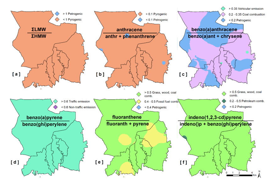
Tobiszewski M, Namiesnik J (2011) PAH diagnostic ratios for the identification of pollution emission sources. Environ Pollut 162: 110–119. https://doi.org/10.1016/J.ENVPOL.2011.10.025 doi: 10.1016/J.ENVPOL.2011.10.025
|
| [91] |
Mostert MMR, Ayoko GA, Kokot S (2010) Application of chemometrics to analysis of soil pollutants. Trends Anal Chem 29: 430–435. https://doi.org/10.1016/j.trac.2010.02.009 doi: 10.1016/j.trac.2010.02.009
|
| [92] |
Zhang W, Zhang S, Wan C, et al. (2008) Source diagnostics of polycyclic aromatic hydrocarbons in urban road runoff, dust, rain and canopy throughfall. Environ Pollut 153: 594–601. https://doi.org/10.1016/j.envpol.2007.09.004 doi: 10.1016/j.envpol.2007.09.004
|
| [93] |
Pies C, Hoffmann B, Petrowsky J, et al. (2008) Characterization and source identification of polycyclic aromatic hydrocarbons (PAHs) in river bank soils. Chemosphere 72: 1594–1601. https://doi.org/10.1016/j.chemosphere.2008.04.021 doi: 10.1016/j.chemosphere.2008.04.021
|
| [94] |
Akyüz M, Çabuk H (2010) Gas and particle partitioning and seasonal variation of polycyclic aromatic hydrocarbons in the atmosphere of Zonguldak, Turkey. Sci Total Environ 408: 5550–5558. https://doi.org/10.1016/j.scitotenv.2010.07.063 doi: 10.1016/j.scitotenv.2010.07.063
|
| [95] |
De La Torre-Roche RJ, Lee W-Y, Campos-Díaz SI (2009) Soil-borne polycyclic aromatic hydrocarbons in El Paso, Texas: analysis of a potential problem in the United States/Mexico border region. J Hazard Mater 163: 946–958. https://doi.org/10.1016/j.jhazmat.2008.07.089 doi: 10.1016/j.jhazmat.2008.07.089
|
| [96] |
Yunker MB, Macdonald RW, Vingarzan R, et al. (2002) PAHs in the Fraser River basin: a critical appraisal of PAH ratios as indicators of PAH source and composition. Org Geochem 33: 489–515. https://doi.org/10.1016/S0146-6380(02)00002-5 doi: 10.1016/S0146-6380(02)00002-5
|
| [97] |
Katsoyiannis A, Terzi E, Cai QY (2007) On the use of PAH molecular diagnostic ratios in sewage sludge for the understanding of the PAH sources. Is this use appropriate? Chemosphere 69: 1337–1339. https://doi.org/10.1016/j.chemosphere.2007.05.084 doi: 10.1016/j.chemosphere.2007.05.084
|
| [98] |
Jiang YF, Wang XT, Jia Y, et al. (2009) Occurrence, distribution and possible sources of organochlorine pesticides in agricultural soil of Shanghai, China. J Hazard Mater 170: 989–997. https://doi.org/10.1016/j.jhazmat.2009.05.082 doi: 10.1016/j.jhazmat.2009.05.082
|
| [99] |
Qiu X, Zhu T, Yao B, et al. (2005) Contribution of dicofol to the current DDT pollution in China. Environ Sci Technol 39: 4385–4390. https://doi.org/10.1021/es050342a doi: 10.1021/es050342a
|
| [100] |
Iwata H, Tanabe S, Ueda K, et al. (1995) Persistent organochlorine residues in Air, Water, Sediments, and Soils from the Lake Baikai Region, Russia. Environ Sci Technol 29: 792–801. https://doi.org/10.1021/es00003a030 doi: 10.1021/es00003a030
|
| [101] |
Zhang ZL, Huang J, Yu G, et al. (2004) Occurrence of PAHs, PCBs and organochlorine pesticides in Tonghui River of Beijing, China. Environ Pollut 130: 249–261. https://doi.org/10.1016/j.envpol.2003.12.002 doi: 10.1016/j.envpol.2003.12.002
|
| [102] |
Zhang A, Liu W, Yuan H, et al. (2011) Spatial distribution of hexachlorocyclohexanes in agricultural soils in Zhejiang province, China, and correlations with elevation and temperature. Environ Sci Technol 45: 6303–6308. https://doi.org/10.1021/es200488n doi: 10.1021/es200488n
|
| [103] |
Bidleman TF, Jantunen LLM, Helm PA, et al. (2000) Chlordane enantiomers and temporal trends of chlordane isomers in Arctic air. Environ Sci Technol 36: 539–544. https://doi.org/10.1021/es011142b doi: 10.1021/es011142b
|
| [104] | WHO, Environmental Health Criteria 40: Endosulfan. World Health Organization, Geneva, 1984. Available from: https://apps.who.int/iris/bitstream/handle/10665/39390/WHO_EHC_40.pdf?sequence=1&isAllowed=y. |
| [105] | Albanese S, Guarino A, Pizzolante A, et al. (2022) The use of natural geochemical background values for the definition of local environmental guidelines: the case study of the Vesuvian plain, In: Baldi D, Uricchio F, Authors, Le bonifiche ambientali nell'ambito della transizione ecologica, Società Italiana di Geologia Ambientale (SIGEA) and Consiglio Nazionale delle Ricerche (CNR), 15–25. |
| [106] |
Aruta A, Albanese S, Daniele L, et al. (2022). A new approach to assess the degree of contamination and determine sources and risks related to PTEs in an urban environment: the case study of Santiago (Chile). Environ Geochem Health. https://doi.org/10.1007/s10653-021-01185-6 doi: 10.1007/s10653-021-01185-6
|
| [107] |
Stančić Z, Fiket Ž, Vuger A (2022) Tin and Antimony as Soil Pollutants along Railway Lines-A Case Study from North-Western Croatia. Environments 9: 10. https://doi.org/10.3390/environments9010010 doi: 10.3390/environments9010010
|
| [108] |
Wuana RA, Okieimen FE (2011) Heavy metals in contaminated soils: a review of sources, chemistry, risks and best available strategies for remediation. Isrn Ecology 2011: 2090–4614. https://doi.org/10.5402/2011/402647 doi: 10.5402/2011/402647
|
| [109] |
Qiu YW, Zhang G, Liu GQ, et al. (2009) Polycyclic aromatic hydrocarbons (PAHs) in the water column and sediment core of Deep Bay, South China. Estuar Coast Shelf Sci 83: 60–66. https://doi.org/10.1016/j.ecss.2009.03.018 doi: 10.1016/j.ecss.2009.03.018
|
| [110] | ATSDR, Toxicological Profile for DDT, DDE, and DDD. Dept Health Human Services. Agency for Toxic Substances and Disease Registry (ATSDR), Atlanta GA, 2002. Available from: https://www.atsdr.cdc.gov/toxprofiles/tp35.pdf. |

Figures(7) / Tables(5)

Stefano Albanese, Annalise Guarino. Assessing contamination sources and environmental hazards for potentially toxic elements and organic compounds in the soils of a heavily anthropized area: the case study of the Acerra plain (Southern Italy)[J]. AIMS Geosciences, 2022, 8(4): 552-578. doi: 10.3934/geosci.2022030


 DownLoad: