The multi-criteria analysis for sustainable urban growth by using Fuzzy Method: case study Trikomo, Cyprus

Can Kara; Nuhcan Akçit; Can Kara; Nuhcan Akçit

doi:10.3934/geosci.2021038

AIMS Geosciences

2021, Volume 7, Issue 4: 623-636. doi: 10.3934/geosci.2021038

Previous Article Next Article

Research article

The multi-criteria analysis for sustainable urban growth by using Fuzzy Method: case study Trikomo, Cyprus

Can Kara ^{1
,
,},
Nuhcan Akçit ²

1.
Department of Architecture, Near East University, Nicosia, Near East Boulevard, Nicosia, North Cyprus, Mersin 10, Turkey
2.
Department of Geodetic and Geographic Information Technology, Middle East Technical University, Ankara, Turkey

Received: 20 August 2021 Accepted: 25 October 2021 Published: 24 November 2021

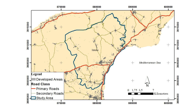
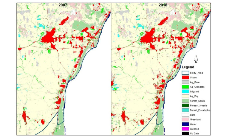
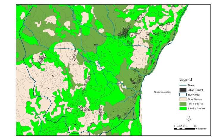
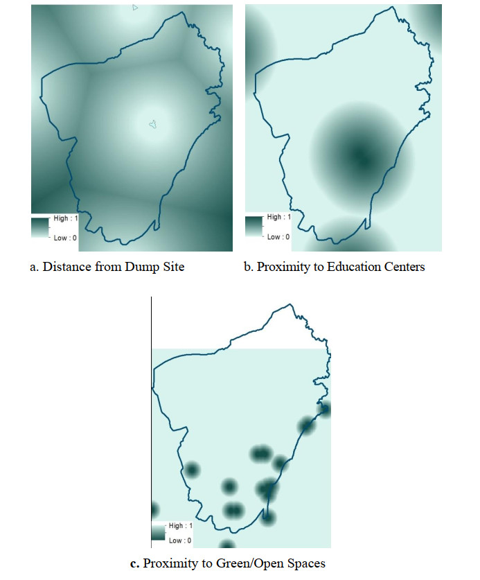
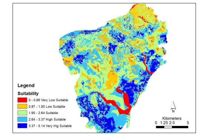
The Urban growth in Trikomo (Yeni İskele) region in Cyprus has dramatically increased recently. The unorganized and uncontrolled development process has started to consume land resources; loss of landcover, valuable agricultural lands, and change of wetlands of stream beds or ponds occurred. In addition, partial and fragmented housing development projects bring only housing and second housing to the coastal region. As a result, environmental and economic problems occurred in sustainable urban growth (SUG) in the Trikomo (Yeni İskele) region. Due to the lack of planning instruments in Trikomo, urban expansion policies and alternatives have been ignored. In this regard, this research tries to investigate spatial SUG and expansion alternatives by using Multi-Criteria Evaluation (MCE) and fuzzy logic within geographical information systems (GIS). Compact growth, environmental protection, and equal accessibility to local services were used for multi-criteria analysis to construct spatial SUG problems. Then they were converted to spatial layers within the (GIS) environment. Results show that; 6 percent of the study area is in a shallow suitability zone. Forty-four percent of it has very low and low suitability for SUG. Also, 41 percent of the area is suitable. Only 12 percent of the area has high and very high suitability values. These findings showed that approximately 118 square kilometers (56 percent) of the city is within the same level appropriate for urban development.

Keywords:

Citation: Can Kara, Nuhcan Akçit. The multi-criteria analysis for sustainable urban growth by using Fuzzy Method: case study Trikomo, Cyprus[J]. AIMS Geosciences, 2021, 7(4): 623-636. doi: 10.3934/geosci.2021038

Related Papers:

[1]	Nadiyah Hussain Alharthi, Abdon Atangana, Badr S. Alkahtani . Numerical analysis of some partial differential equations with fractal-fractional derivative. AIMS Mathematics, 2023, 8(1): 2240-2256. doi: 10.3934/math.2023116
[2]	Hasib Khan, Jehad Alzabut, Anwar Shah, Sina Etemad, Shahram Rezapour, Choonkil Park . A study on the fractal-fractional tobacco smoking model. AIMS Mathematics, 2022, 7(8): 13887-13909. doi: 10.3934/math.2022767
[3]	Abdon Atangana, Seda İğret Araz . Extension of Chaplygin's existence and uniqueness method for fractal-fractional nonlinear differential equations. AIMS Mathematics, 2024, 9(3): 5763-5793. doi: 10.3934/math.2024280
[4]	Manal Alqhtani, Khaled M. Saad . Numerical solutions of space-fractional diffusion equations via the exponential decay kernel. AIMS Mathematics, 2022, 7(4): 6535-6549. doi: 10.3934/math.2022364
[5]	Abdon Atangana, Ali Akgül . Analysis of a derivative with two variable orders. AIMS Mathematics, 2022, 7(5): 7274-7293. doi: 10.3934/math.2022406
[6]	Emile Franc Doungmo Goufo, Abdon Atangana . On three dimensional fractal dynamics with fractional inputs and applications. AIMS Mathematics, 2022, 7(2): 1982-2000. doi: 10.3934/math.2022114
[7]	Rahat Zarin, Amir Khan, Pushpendra Kumar, Usa Wannasingha Humphries . Fractional-order dynamics of Chagas-HIV epidemic model with different fractional operators. AIMS Mathematics, 2022, 7(10): 18897-18924. doi: 10.3934/math.20221041
[8]	Muhammad Farman, Ali Akgül, Kottakkaran Sooppy Nisar, Dilshad Ahmad, Aqeel Ahmad, Sarfaraz Kamangar, C Ahamed Saleel . Epidemiological analysis of fractional order COVID-19 model with Mittag-Leffler kernel. AIMS Mathematics, 2022, 7(1): 756-783. doi: 10.3934/math.2022046
[9]	Amir Ali, Abid Ullah Khan, Obaid Algahtani, Sayed Saifullah . Semi-analytical and numerical computation of fractal-fractional sine-Gordon equation with non-singular kernels. AIMS Mathematics, 2022, 7(8): 14975-14990. doi: 10.3934/math.2022820
[10]	Muhammad Aslam, Muhammad Farman, Hijaz Ahmad, Tuan Nguyen Gia, Aqeel Ahmad, Sameh Askar . Fractal fractional derivative on chemistry kinetics hires problem. AIMS Mathematics, 2022, 7(1): 1155-1184. doi: 10.3934/math.2022068

Abstract

1. Introduction, definitions and preliminaries

Fractional calculus is a generalization of classical calculus and many researchers have paid attention to this science as they encounter many of these issues in the real world. Most of these issues do not have analytical exact solution. Which made many researchers interest and search in numerical and approximate methods to obtain solutions using these methods. There are many of these methods, such as the homotopy analysis ^[1,2,3,4], He's variational iteration method ^[5,6], Adomians decomposition method ^[7,8,9], Fourier spectral methods ^[10], finite difference schemes ^[11], collocation methods ^[12,13,14]. To find out more about the fractal calculus, refer to the following references ^[15,16]. More recently, a new concept was introduced for the fractional operator, as this operator has two orders, the first representing the fractional order, and the second representing the fractal dimension. In our work we aim to applied the idea of fractal-fractional derivative of orders $\beta, k$ to a reaction-diffusion equation with $q$ -th nonlinear. To this end ^[17], we replace the derivative with respect to t by the fractal-fractional derivatives power (FFP) law, the fractal-fractional exponential(FFE) law and the fractal-fractional Mittag-Leffler (FFM) law kernels which corresponds to the ^[18], Caputo-Fabrizio (CF) ^[19] and the Atangana-Baleanu (AB) ^[20] fractional derivatives, respectively. This topic has attracted many researchers and has been applied to research related to the real world, such as ^{[21,22,23,24,25,26]}. Some recent developments in the area of numerical techniques can be found in ^{[27,28,29,30,31]}.

Merkin and Needham ^[32] considered the reaction-diffusion travelling waves that can develop in a coupled system involving simple isothermal autocatalysis kinetics. They assumed that reactions took place in two separate and parallel regions, with, in $I$ , the reaction being given by quadratic autocatalysis

$\begin{equation} F + G \rightarrow 2G( \text{rate}\, k_{1}f\, g), \end{equation}$

(1.1)

together with a linear decay step

$\begin{equation} G \rightarrow H( \text{rate}\, k_{2}\, g) \end{equation}$

(1.2)

where $f$ and $g$ are the concentrations of reactant $F$ and autocatalyst $H$ , the $k_{i}(i = 1, 2)$ are the rate constants and $H$ is some inert product of reaction. The reaction in region $II$ was the quadratic autocatalytic step (1.1) only. The two regions were assumed to be coupled via a linear diffusive interchange of the autocatalytic species $G$ . We shall consider a similar system as I, but with cubic autocatalysis

$\begin{equation} F+ 2G \rightarrow 3G( \text{rate}\, k_{3}\, f g^{2}) \end{equation}$

(1.3)

together with a linear decay step

$\begin{equation} G \rightarrow H( \text{rate}\, k_{4}g). \end{equation}$

(1.4)

For $q$ -th autocatalytic, we have

$\begin{equation} F+ q G \rightarrow (q+1)G ( \text{rate} \, k_{3}f g^{q}), \, \, 1 \leq q \leq 2, \end{equation}$

(1.5)

together with a linear decay step

$\begin{equation} G \rightarrow H( \text{rate }\, k_{4} g). \end{equation}$

(1.6)

This yields to the following system

$\begin{equation} \frac{\partial \eta_{1}}{\partial t} = \frac{\partial^{2}\eta_{1}}{\partial \xi^{2}}+\nu(\eta_{2}-\eta_{1})-\eta_{1} \zeta_{1}^{q}, \end{equation}$

(1.7)

$\begin{equation} \frac{\partial \zeta_{1}}{\partial t} = \frac{\partial^{2}\zeta_{1}}{\partial \xi^{2}}-\kappa \zeta_{1}+\eta_{1} \zeta_{1}^{q}, \end{equation}$

(1.8)

$\begin{equation} \frac{\partial \eta_{2}}{\partial t} = \frac{\partial^{2}\eta_{2}}{\partial \xi^{2}}+ \nu(\eta_{1}-\eta_{2})-\eta_{2} \zeta_{2}^{q}, \end{equation}$

(1.9)

$\begin{equation} \frac{\partial \zeta_{2}}{\partial t} = \frac{\partial^{2}\zeta_{2}}{\partial \xi^{2}}+\eta_{2} \zeta_{2}^{q} \end{equation}$

(1.10)

where $\nu$ represents the couple between (I) and (II) and $\kappa$ represents the strength of the auto-catalyst decay. For more details see ^[32]. Omitting the diffusion terms in the system (1.7)-(1.10), one has the following ordinary differential equations

$\begin{equation} \frac{\partial \eta_{1}}{\partial t} = \nu(\eta_{2}-\eta_{1})-\eta_{1} \zeta_{1}^{q}, \end{equation}$

(1.11)

$\begin{equation} \frac{\partial \zeta_{1}}{\partial t} = -\kappa \zeta_{1}+\eta_{1} \zeta_{1}^{q}, \end{equation}$

(1.12)

$\begin{equation} \frac{\partial \eta_{2}}{\partial t} = \nu(\eta_{1}-\eta_{2})-\eta_{2} \zeta_{2}^{q}, \end{equation}$

(1.13)

$\begin{equation} \frac{\partial \zeta_{2}}{\partial t} = \eta_{2} \zeta_{2}^{q}. \end{equation}$

(1.14)

Now we provide some basic definitions that be needed in this work. As for the theorems and proofs related to the three fractal-fractional operators, they are found in details in ^[17]. Thus we suffice in this work by constructing the algorithms and making the numerical simulations of the set of Eqs (1.7)-(1.10) with the three fractal-fractional operators.

Definition 1. If $\eta(t)$ is continuous and fractal differentiable on $(a, b)$ of order $k$ , then the fractal-fractional derivative of $\eta(t)$ of order $\beta$ in Riemann Liouville sense with the power law is given by ^[17]:

$\begin{align} ^ \text{{FFP}}_{0}D_{t}^{\beta, \, k}\eta(t)& = \frac{1}{\Gamma(1-\beta)}\frac{d}{dt^{k}} \int_{0}^{t}(t-\tau)^{-\beta}\eta(\tau) d\tau, \, \, \, \, (0 \lt \beta, \, k \leq1), \end{align}$

(1.15)

and the fractal-fractional integral of $\eta(t)$ is given by

$\begin{align} ^{ \text{FFP}}_{\;\;\;\;\;0}{I}_t^{\beta, \, k}\eta(t) = \frac{k}{\Gamma(\beta)}\int_{0}^{t}\tau^{k-1}(t - \tau)^{\beta-1} \eta(\tau) d\tau. \end{align}$

(1.16)

Definition 2. If $\eta(t)$ is continuous in the $(a, b)$ and fractal differentiable on $(a, b)$ with order $k$ , then the fractal-fractional derivative of $\eta(t)$ of order $\beta$ in Riemann Liouville sense with the exponential decay kernel is given by ^[17]:

$\begin{align} ^{ \text{FFE}}_{0}D_{t}^{\beta, k}\eta(t)& = \frac{M(\beta)}{1-\beta}\frac{d}{dt^{k}} \int_{0}^{t} e^{\frac{-\beta}{1-\beta}(t-\tau)}\eta(\tau) d\tau, \, \, \, \, (0 \lt \beta, \, k \leq1), \end{align}$

(1.17)

and the fractal-fractional integral of $\eta(t)$ is given by

$\begin{align} ^{ \text{FFE}}_{\;\;\;\;\;0}{I}_t^{\beta, k}\eta(t) = \frac{(1-\beta) k t^{k-1}}{ M(\beta)} \eta(t)+\frac{\beta k}{M(\beta)}\int_{0}^{t}\tau^{k-1} \eta(\tau) d\tau \end{align}$

(1.18)

where $M(\beta)$ is the normalization function such that $M(0) = M(1) = 1.$

Definition 3. If $\eta(t)$ is continuous in the $(a, b)$ and fractal differentiable on $(a, b)$ with order $k$ , then the fractal-fractional derivative of $\eta(t)$ of order $\beta$ in Riemann Liouville sense with the Mittag-Leffler type kernel is given by ^[17]:

$\begin{align} ^{FFE}_{0}D_{t}^{\beta, k}\eta(t)& = \frac{A(\beta)}{1-\beta}\frac{d}{dt^{k}} \int_{0}^{t} E_{\beta}\Big({\frac{-\beta}{1-\beta}(t-\tau)}\Big)\eta(\tau) d\tau, \, \, \, \, (0 \lt \beta, \, k \leq1), \end{align}$

(1.19)

and the fractal-fractional integral of $\eta(t)$ is given by

$\begin{align} ^{ \text{FFE}}_{\;\;\;\;\;0}{I}_t^{\beta, k}\eta(t) = \frac{(1-\beta) k t^{k-1}}{ A(\beta)} \eta(t)+\frac{\beta \, k}{A(\beta) \Gamma(\beta)}\int_{0}^{t}\tau^{k-1} (t-\tau)^{\beta-1} \eta(\tau) d\tau, \end{align}$

(1.20)

$\begin{align} \frac{d\eta(t)}{dt^{k}} = lim_{\tau\rightarrow t}\frac{\eta(\tau)-\eta(t)}{\tau^{k}-t^{k}} \end{align}$

(1.21)

where where $A(\beta) = 1-\beta+\dfrac{\beta}{\Gamma(\beta)}$ is a normalization function such that $A(0) = A(1) = 1$ .

Our contribution to this paper is to construct the successive approximations and evaluate the numerical solutions of the FFRDE. These successive approximations allow us to study the behavior of numerical solutions based on power, exponential, and the Mittag-Leffler kernels. Also we can study the behavior of approximate solutions in the case of nonlinearity of the FFRDE in general. To our best knowledge, this is the first study of the FFRDE using fractal-fractional with these kernels. The importance of these results lies in the fact that they highlight the possibility of using these results for the benefit of chemical and physical researchers, by trying to link the numerical results of these mathematical models with the laboratory results. These results also contribute to the reliance on numerical results in the case of many models related to the real world, which often cannot find an analytical solution. The structure of this paper is summarized as follows: In sections, two, three and four, the FFRDE is presented with the three kernels that proposed in this work and construct the successive approximations. In section Five, numerical solutions for the FFRDE are discussed with a study of their behavior. Section Six the conclusion is presented.

2. Numerical scheme of FFRDE of q-th-order autocatalysis due the power law kernel

The new model is obtained by replacing the ordinary derivative with the the fractal-fractional derivative the power law kernel as ^[17]

$\begin{align} ^{ \text{FFP}}_{0}D_{t}^{\beta}\eta_{1}(t) = \nu(\eta_{2}(t)-\eta_{1}(t))-\eta_{1}(t) \zeta_{1}^{q}(t), \end{align}$

(2.1)

$\begin{align} ^{ \text{FFP}}_{0}D_{t}^{\beta}\zeta_{1}(t) = -\kappa \zeta_{1}(t)+\eta_{1}(t) \zeta_{1}^{q}(t), \end{align}$

(2.2)

$\begin{align} ^{ \text{FFP}}_{0}D_{t}^{\beta}\eta_{2}(t) = \nu(\eta_{1}(t)-\eta_{2}(t))-\eta_{2}(t) \zeta_{2}^{q}(t), \end{align}$

(2.3)

$\begin{align} ^{ \text{FFP}}_{0}D_{t}^{\beta}\zeta_{2}(t) = \eta_{2}(t) \zeta_{2}^{q}(t). \end{align}$

(2.4)

By following the procedure in ^[17], we can obtain the following successive approximations:

$\begin{align} \eta_{1}(t) - \eta_{1}(0) & = \frac{k}{\Gamma(\beta)} \int_{0}^{t} \tau^{k-1} (t - \tau)^{\beta - 1} \varphi_{1}(\eta_{1}, \zeta_{1}, \eta_{2}, \zeta_{2}, \tau)d\tau, \end{align}$

(2.5)

$\begin{align} \zeta_{1}(t) - \zeta_{2}(0) & = \frac{k}{\Gamma(\beta)} \int_{0}^{t} \tau^{k-1} (t - \tau)^{\beta - 1} \varphi_{2}(\eta_{1}, \zeta_{1}, \eta_{2}, \zeta_{2}, \tau)d\tau, \end{align}$

(2.6)

$\begin{align} \eta_{2}(t) - \eta_{3}(0) & = \frac{k}{\Gamma(\beta)} \int_{0}^{t} \tau^{k-1}(t - \tau)^{\beta - 1} \varphi_{3}(\eta_{1}, \zeta_{1}, \eta_{2}, \zeta_{2}, \tau)d\tau, \end{align}$

(2.7)

$\begin{align} \zeta_{2}(t) - \zeta_{2}(0) & = \frac{k}{\Gamma(\beta)} \int_{0}^{t} \tau^{k-1} (t - \tau)^{\beta - 1}\varphi_{4}(\eta_{1}, \zeta_{1}, \eta_{2}, \zeta_{2}, \tau) d\tau \end{align}$

(2.8)

where

$\begin{align} \varphi_{1}(\eta_{1}, \zeta_{1}, \eta_{2}, \zeta_{2}, \tau)& = \Big(\nu\, (\eta_{2}(\tau)-\eta_{1}(\tau))-\eta_{1}(\tau) \zeta_{1}^{q}(\tau)\Big), \end{align}$

(2.9)

$\begin{align} \varphi_{2}(\eta_{1}, \zeta_{1}, \eta_{2}, \zeta_{2}, \tau)& = \Big( -\kappa \, \zeta_{1}(\tau)+\eta_{1}(\tau) \zeta_{1}^{q}(\tau)\Big), \end{align}$

(2.10)

$\begin{align} \varphi_{3}(\eta_{1}, \zeta_{1}, \eta_{2}, \zeta_{2}, \tau)& = \Big(\nu(\eta_{1}(\tau)-\eta_{2}(\tau))-\eta_{2}(\tau) \zeta_{2}^{q}(\tau)\Big), \end{align}$

(2.11)

$\begin{align} \varphi_{4}(\eta_{1}, \zeta_{1}, \eta_{2}, \zeta_{2}, \tau)& = \eta_{2}(\tau) \zeta_{2}^{q}(\tau). \end{align}$

(2.12)

Equation (2.5)-(2.8) can be reformulated as

$\begin{equation} \eta_{1}(t) - \eta_{1}(0) = \frac{k}{\Gamma(\beta)}\sum\limits_{m = 0}^{n} \int_{t_{m}}^{t_{m+1}} \tau^{k-1} (t_{n+1} - \tau)^{\beta - 1} \varphi_{1}(\eta_{1}, \zeta_{1}, \eta_{2}, \zeta_{2}, \tau)d\tau, \end{equation}$

(2.13)

$\begin{equation} \zeta_{1}(t) - \zeta_{1}(0) = \frac{k}{\Gamma(\beta)}\sum\limits_{m = 0}^{n} \int_{t_{m}}^{t_{m+1}} \tau^{k-1} (t_{n+1} - \tau)^{\beta - 1} \varphi_{2}(\eta_{1}(\tau), \zeta_{1}(\tau), \eta_{2}(\tau), \zeta_{2}(\tau), \tau)d\tau, \end{equation}$

(2.14)

$\begin{equation} \eta_{2}(t) - \eta_{2}(0) = \frac{k}{\Gamma(\beta)} \sum\limits_{m = 0}^{n} \int_{t_{m}}^{t_{m+1}} \tau^{k-1}(t_{n+1} - \tau)^{\beta - 1} \varphi_{3}(\eta_{1}, \zeta_{1}, \eta_{2}, \zeta_{2}, \tau)d\tau, \end{equation}$

(2.15)

$\begin{equation} \zeta_{2}(t) - \zeta_{2}(0) = \frac{k}{\Gamma(\beta)} \sum\limits_{m = 0}^{n} \int_{t_{m}}^{t_{m+1}} \tau^{k-1} (t_{n+1} - \tau)^{\beta - 1}\varphi_{4}(\eta_{1}, \zeta_{1}, \eta_{2}, \zeta_{2}, \tau)d\tau. \end{equation}$

(2.16)

Using the two-step Lagrange polynomial interpolation, we obtain

$\begin{align} \eta_{1}(t) - \eta_{1}(0) & = \frac{k}{\Gamma(\beta)}\sum\limits_{m = 0}^{n} \int_{t_{m}}^{t_{m+1}} (t_{n+1} - \tau)^{\beta - 1} Q_{1, m}(\tau)d\tau, \end{align}$

(2.17)

$\begin{align} \zeta_{1}(t) - \zeta_{1}(0) & = \frac{k}{\Gamma(\beta)}\sum\limits_{m = 0}^{n} \int_{t_{m}}^{t_{m+1}} (t_{n+1} - \tau)^{\beta - 1} Q_{2, m}(\tau)d\tau, \end{align}$

(2.18)

$\begin{align} \eta_{2}(t) - \eta_{2}(0) & = \frac{k}{\Gamma(\beta)} \sum\limits_{m = 0}^{n} \int_{t_{m}}^{t_{m+1}} (t_{n+1} - \tau)^{\beta - 1}Q_{3, m}(\tau)d\tau, \end{align}$

(2.19)

$\begin{align} \zeta_{2}(t) - \zeta_{2}(0) & = \frac{k}{\Gamma(\beta)} \sum\limits_{m = 0}^{n} \int_{t_{m}}^{t_{m+1}} (t_{n+1} - \tau)^{\beta - 1}Q_{4, m}(\tau) d\tau, \end{align}$

(2.20)

where,

$\begin{align} Q_{1, m}(\tau)& = \frac{\tau-t_{m-1}}{t_{m}-t_{m-1}}t^{k-1}_{m}\varphi_{1}(\eta_{1}(\tau_{m}), \zeta_{1}(\tau_{m}), \eta_{2}(\tau_{m}), \zeta_{2}(\tau_{m}), \tau_{m})-\frac{\tau-t_{m}}{t_{m}-t_{m-1}}\\ \times&t^{k-1}_{m-1}\varphi_{1}(\eta_{1}(\tau_{m-1}), \zeta_{1}(\tau_{m-1}), \eta_{2}(\tau_{m-1}), \zeta_{2}(\tau_{m-1}), \tau_{m-1}), \end{align}$

(2.21)

$\begin{align} Q_{2, m}(\tau)& = \frac{\tau-t_{m-1}}{t_{m}-t_{m-1}}t^{k-1}_{m}\varphi_{2}(\eta_{1}(\tau_{m}), \zeta_{1}(\tau_{m}), \eta_{2}(\tau_{m}), \zeta_{2}(\tau_{m}), \tau_{m})-\frac{\tau-t_{m}}{t_{m}-t_{m-1}}\\ \times&t^{k-1}_{m-1}\varphi_{2}(\eta_{1}(\tau_{m-1}), \zeta_{1}(\tau_{m-1}), \eta_{2}(\tau_{m-1}), \zeta_{2}(\tau_{m-1}), \tau_{m-1}), \end{align}$

(2.22)

$\begin{align} Q_{3, m}(\tau)& = \frac{\tau-t_{m-1}}{t_{m}-t_{m-1}}t^{k-1}_{m}\varphi_{3}(\eta_{1}(\tau_{m}), \zeta_{1}(\tau_{m}), \eta_{2}(\tau_{m}), \zeta_{2}(\tau_{m}), \tau_{m})-\frac{\tau-t_{m}}{t_{m}-t_{m-1}}\\ \times&t^{k-1}_{m-1}\varphi_{3}(\eta_{1}(\tau_{m-1}), \zeta_{1}(\tau_{m-1}), \eta_{2}(\tau_{m-1}), \zeta_{2}(\tau_{m-1}), \tau_{m-1}), \end{align}$

(2.23)

$\begin{align} Q_{4, m}(\tau)& = \frac{\tau-t_{m-1}}{t_{m}-t_{m-1}}t^{k-1}_{m}\varphi_{4}(\eta_{4}(\tau_{m}), \zeta_{1}(\tau_{m}), \eta_{2}(\tau_{m}), \zeta_{2}(\tau_{m}), \tau_{m})-\frac{\tau-t_{m}}{t_{m}-t_{m-1}}\\ \times&t^{k-1}_{m-1}\varphi_{4}(\eta_{1}(\tau_{m-1}), \zeta_{1}(\tau_{m-1}), \eta_{2}(\tau_{m-1}), \zeta_{2}(\tau_{m-1}), \tau_{m-1}). \end{align}$

(2.24)

These integrals are evaluated directly and the numerical solutions of (2.1)-(2.4) involving the FFP derivative are given by

$\begin{eqnarray} \eta_{1}(t_{n+1}) & = & \eta_{1}(0) + \frac{k h^{\beta}}{\Gamma(\beta+2)} \sum\limits_{m = 0}^{n} t^{k-1}_{m} \varphi_{1}(\eta_{1}(t_{m}), \zeta_{1}(t_{m}), \eta_{2}(t_{m}), \zeta_{2}(t_{m}), t_{m})\Xi_{1}(n, m) \\ &-&t^{k-1}_{m-1}\varphi_{1}(\eta_{1}(\tau_{m-1}), \zeta_{1}(t_{m-1}), \eta_{2}(t_{m-1}), \zeta_{2}(t_{m-1}), t_{m-1})\Xi_{2}(n, m)\Big), \end{eqnarray}$

(2.25)

$\begin{eqnarray} \zeta_{1}(t_{n+1}) & = & \zeta_{1}(0) + \frac{k h^{\beta}}{\Gamma(\beta+2)} \sum\limits_{m = 0}^{n} t^{k-1}_{m} \varphi_{2}(\eta_{1}(t_{m}), \zeta_{1}(t_{m}), \eta_{2}(t_{m}), \zeta_{2}(t_{m}), t_{m})\Xi_{1}(n, m) \\ &-&t^{k-1}_{m-1}\varphi_{2}(\eta_{1}(\tau_{m-1}), \zeta_{1}(t_{m-1}), \eta_{2}(t_{m-1}), \zeta_{2}(t_{m-1}), t_{m-1})\Xi_{2}(n, m)\Big), \end{eqnarray}$

(2.26)

$\begin{eqnarray} \eta_{2}(t_{n+1}) & = & \eta_{2}(0) + \frac{k h^{\beta}}{\Gamma(\beta+2)} \sum\limits_{m = 0}^{n} t^{k-1}_{m} \varphi_{3}(\eta_{1}(t_{m}), \zeta_{1}(t_{m}), \eta_{2}(t_{m}), \zeta_{2}(t_{m}), t_{m})\Xi_{1}(n, m) \\ &-&t^{k-1}_{m-1}\varphi_{4}(\eta_{1}(\tau_{m-1}), \zeta_{1}(t_{m-1}), \eta_{2}(t_{m-1}), \zeta_{2}(t_{m-1}), t_{m-1})\Xi_{2}(n, m)\Big), \end{eqnarray}$

(2.27)

$\begin{eqnarray} \zeta_{2}(t_{n+1}) & = & \zeta_{2}(0) + \frac{k h^{\beta}}{\Gamma(\beta+2)} \sum\limits_{m = 0}^{n} t^{k-1}_{m} \varphi_{4}(\eta_{1}(t_{m}), \zeta_{1}(t_{m}), \eta_{2}(t_{m}), \zeta_{2}(t_{m}), t_{m})\Xi_{1}(n, m) \\ &-&t^{k-1}_{m-1}\varphi_{4}(\eta_{1}(\tau_{m-1}), \zeta_{1}(t_{m-1}), \eta_{2}(t_{m-1}), \zeta_{2}(t_{m-1}), t_{m-1})\Xi_{2}(n, m)\Big), \end{eqnarray}$

(2.28)

$\begin{equation} \begin{aligned} \Xi_{1}(n, m)& = \Big((n + 1 - m)^{\beta}(n -m + 2 + \beta) - (n - m)^{\beta}\times (n -m + 2 + 2\beta) \Big), \end{aligned} \end{equation}$

(2.29)

$\begin{equation} \begin{aligned} \Xi_{2}(n, m) = \Big((n + 1 - m)^{\beta+1} - (n -m)^{\beta}(n -m + 1 + \beta)\Big). \end{aligned} \end{equation}$

(2.30)

3. Numerical scheme of FFRDE of $q$ -th-order autocatalysis due the exponential decay kernel

Considering the FFE derivative, we have from ^[17]

$\begin{align} ^{ \text{FFE}}_{0}D_{t}^{\beta}\eta_{1}(t) = \nu(\eta_{2}(t)-\eta_{1}(t))-\eta_{1}(t) \zeta_{1}^{q}(t), \end{align}$

(3.1)

$\begin{align} ^{ \text{FFE}}_{0}D_{t}^{\beta}\zeta_{1}(t) = -\kappa \zeta_{1}(t)+\eta_{1}(t) \zeta_{1}^{q}(t), \end{align}$

(3.2)

$\begin{align} ^{ \text{FFE}}_{0}D_{t}^{\beta}\eta_{2}(t) = \nu(\eta_{1}(t)-\eta_{2}(t))-\eta_{2}(t) \zeta_{2}^{q}(t), \end{align}$

(3.3)

$\begin{align} ^{ \text{FFE}}_{0}D_{t}^{\beta}\zeta_{2}(t) = \eta_{2}(t) \zeta_{2}^{q}(t). \end{align}$

(3.4)

For the successive approximations of the system (3.1)-(3.4), we follow the same procedures as in ^[17], we obtain

$\begin{eqnarray} \eta_{1}(t)- \eta_{1}(0) & = & \frac{k t^{k-1}(1 - \beta)}{M(\beta)} \varphi_{1}(\eta_{1}, \zeta_{1}, \eta_{2}, \zeta_{2}, t) \\ &+& \frac{\beta}{M(\beta)} \int_{0}^{t} k\, \tau^{k-1}\varphi_{1}(\eta_{1}, \zeta_{1}, \eta_{2}, \zeta_{2}, \tau) d\tau, \end{eqnarray}$

(3.5)

$\begin{eqnarray} \zeta_{1}(t)- \zeta_{1}(0) & = & \frac{k t^{k-1}(1 - \beta)}{M(\beta)} \varphi_{2}(\eta_{1}, \zeta_{1}, \eta_{2}, \zeta_{2}, t) \\ &+& \frac{\beta}{M(\beta)} \int_{0}^{t} k\, \tau^{k-1}\varphi_{2}(\eta_{1}, \zeta_{1}, \eta_{2}, \zeta_{2}, \tau) d\tau, \end{eqnarray}$

(3.6)

$\begin{eqnarray} \eta_{2}(t)- \eta_{2}(0) & = & \frac{k t^{k-1}(1 - \beta)}{M(\beta)} \varphi_{3}(\eta_{1}, \zeta_{1}, \eta_{2}, \zeta_{2}, t) \\ &+& \frac{\beta}{M(\beta)} \int_{0}^{t} k\, \tau^{k-1}\varphi_{3}(\eta_{1}, \zeta_{1}, \eta_{2}, \zeta_{2}, \tau) d\tau, \end{eqnarray}$

(3.7)

$\begin{eqnarray} \zeta_{2}(t)- \zeta_{2}(0) & = & \frac{k t^{k-1}(1 - \beta)}{M(\beta)} \varphi_{4}(\eta_{1}, \zeta_{1}, \eta_{2}, \zeta_{2}, t) \\ &+& \frac{\beta}{M(\beta)} \int_{0}^{t} k\, \tau^{k-1}\varphi_{4}(\eta_{1}, \zeta_{1}, \eta_{2}, \zeta_{2}, \tau) d\tau. \end{eqnarray}$

(3.8)

Using $t = t_{n+1}$ the following is established

$\begin{eqnarray} \eta_{1}(t_{n+1})- \eta_{1}(0) & = & \frac{k t^{k-1}(1 - \beta)}{M(\beta)} \varphi_{1}(\eta_{1}, \zeta_{1}, \eta_{2}, \zeta_{2}, t_{n}) \\ &+& \frac{\beta}{M(\beta)} \int_{0}^{t_{n+1}} k\, \tau^{k-1}\varphi_{1}(\eta_{1}, \zeta_{1}, \eta_{2}, \zeta_{2}, \tau) d\tau, \end{eqnarray}$

(3.9)

$\begin{eqnarray} \zeta_{1}(t_{n+1})- \zeta_{1}(0) & = & \frac{k t^{k-1}(1 - \beta)}{M(\beta)} \varphi_{2}(\eta_{1}, \zeta_{1}, \eta_{2}, \zeta_{2}, t_{n}) \\ &+& \frac{\beta}{M(\beta)} \int_{0}^{t_{n+1}} k\, \tau^{k-1}\varphi_{2}(\eta_{1}, \zeta_{1}, \eta_{2}, \zeta_{2}, \tau) d\tau, \end{eqnarray}$

(3.10)

$\begin{eqnarray} \eta_{2}(t_{n+1})- \eta_{2}(0) & = & \frac{k t^{k-1}(1 - \beta)}{M(\beta)} \varphi_{3}(\eta_{1}, \zeta_{1}, \eta_{2}, \zeta_{2}, t_{n}) \\ &+& \frac{\beta}{M(\beta)} \int_{0}^{t_{n+1}} k\, \tau^{k-1}\varphi_{3}(\eta_{1}, \zeta_{1}, \eta_{2}, \zeta_{2}, \tau) d\tau, \end{eqnarray}$

(3.11)

$\begin{eqnarray} \zeta_{2}(t_{n+1})- \zeta_{2}(0) & = & \frac{k t^{k-1}(1 - \beta)}{M(\beta)} \varphi_{4}(\eta_{1}, \zeta_{1}, \eta_{2}, \zeta_{2}, t_{n}) \\ &+& \frac{\beta}{M(\beta)} \int_{0}^{t_{n+1}} k\, \tau^{k-1}\varphi_{4}(\eta_{1}, \zeta_{1}, \eta_{2}, \zeta_{2}, \tau) d\tau. \end{eqnarray}$

(3.12)

Further, we have the following:

$\begin{eqnarray} \eta_{1}(t_{n+1})- \eta_{1}(t_{n}) & = & \frac{k t^{k-1}_{n}(1 - \beta)}{M(\beta)} \varphi_{1}(\eta_{1}, \zeta_{1}, \eta_{2}, \zeta_{2}, t_{n}) \\ &-&\frac{k t^{k-1}_{n-1}(1 - \beta)}{M(\beta)}\varphi_{1}(\eta_{1}, \zeta_{1}, \eta_{2}, \zeta_{2}, t_{n-1}) \\ &+& \frac{\beta}{M(\beta)} \int_{t_{n}}^{t_{n+1}} k\, \tau^{k-1}\varphi_{1}(\eta_{1}, \zeta_{1}, \eta_{2}, \zeta_{2}, \tau) d\tau, \end{eqnarray}$

(3.13)

$\begin{eqnarray} \zeta_{1}(t_{n+1})- \zeta_{1}(t_{n}) & = & \frac{k t^{k-1}_{n}(1 - \beta)}{M(\beta)} \varphi_{2}(\eta_{1}, \zeta_{1}, \eta_{2}, \zeta_{2}, t_{n}) \\ &-&\frac{k t^{k-1}_{n-1}(1 - \beta)}{M(\beta)}\varphi_{2}(\eta_{1}, \zeta_{1}, \eta_{2}, \zeta_{2}, t_{n-1}) \\ &+& \frac{\beta}{M(\beta)} \int_{t_{n}}^{t_{n+1}} k\, \tau^{k-1}\varphi_{2}(\eta_{1}, \zeta_{1}, \eta_{2}, \zeta_{2}, \tau) d\tau, \end{eqnarray}$

(3.14)

$\begin{eqnarray} \eta_{2}(t_{n+1})- \eta_{2}(t_{n}) & = & \frac{k t^{k-1}_{n}(1 - \beta)}{M(\beta)} \varphi_{3}(\eta_{1}, \zeta_{1}, \eta_{2}, \zeta_{2}, t_{n}) \\ &-&\frac{k t^{k-1}_{n-1}(1 - \beta)}{M(\beta)}\varphi_{3}(\eta_{1}, \zeta_{1}, \eta_{2}, \zeta_{2}, t_{n-1}) \\ &+& \frac{\beta}{M(\beta)} \int_{t_{n}}^{t_{n+1}} k\, \tau^{k-1}\varphi_{3}(\eta_{1}, \zeta_{1}, \eta_{2}, \zeta_{2}, \tau) d\tau, \end{eqnarray}$

(3.15)

$\begin{eqnarray} \zeta_{2}(t_{n+1})- \zeta_{2}(t_{n}) & = & \frac{k t^{k-1}_{n}(1 - \beta)}{M(\beta)} \varphi_{4}(\eta_{1}, \zeta_{1}, \eta_{2}, \zeta_{2}, t_{n}) \\ &-&\frac{k t^{k-1}_{n-1}(1 - \beta)}{M(\beta)}\varphi_{4}(\eta_{1}, \zeta_{1}, \eta_{2}, \zeta_{2}, t_{n-1}) \\ &+& \frac{\beta}{M(\beta)} \int_{t_{n}}^{t_{n+1}} k\, \tau^{k-1}\varphi_{4}(\eta_{1}, \zeta_{1}, \eta_{2}, \zeta_{2}, \tau) d\tau. \end{eqnarray}$

(3.16)

It follows from the Lagrange polynomial interpolation and integrating the following expressions:

$\begin{eqnarray} \eta_{1}(t_{n+1})- \eta_{1}(t_{n}) & = & \frac{k t^{k-1}_{n}(1 - \beta)}{M(\beta)} \varphi_{1}(\eta_{1}, \zeta_{1}, \eta_{2}, \zeta_{2}, t_{n}) \\ &-&\frac{k t^{k-1}_{n-1}(1 -\beta)}{M(\beta)} \varphi_{1}(\eta_{1}, \zeta_{1}, \eta_{2}, \zeta_{2}, t_{n-1}) +\frac{k h \beta }{2 M(\beta)} \\ &\times& \Big(3 t^{k-1}_{n}\varphi_{1}(\eta_{1}, \zeta_{1}, \eta_{2}, \zeta_{2}, t_{n}) -t^{k-1}_{n-1}\varphi_{1}(\eta_{1}, \zeta_{1}, \eta_{2}, \zeta_{2}, t_{n-1}) , \end{eqnarray}$

(3.17)

$\begin{eqnarray} \zeta_{1}(t_{n+1})- \zeta_{1}(t_{n}) & = & \frac{k t^{k-1}_{n}(1 - \beta)}{M(\beta)} \varphi_{2}(\eta_{1}, \zeta_{1}, \eta_{2}, \zeta_{2}, t_{n}) \\ &-&\frac{k t^{k-1}_{n-1}(1 -\beta)}{M(\beta)} \varphi_{2}(\eta_{1}, \zeta_{1}, \eta_{2}, \zeta_{2}, t_{n-1}) +\frac{k h \beta }{2 M(\beta)} \\ &\times& \Big(3 t^{k-1}_{n}\varphi_{2}(\eta_{1}, \zeta_{1}, \eta_{2}, \zeta_{2}, t_{n}) -t^{k-1}_{n-1}\varphi_{2}(\eta_{1}, \zeta_{1}, \eta_{2}, \zeta_{2}, t_{n-1}) , \end{eqnarray}$

(3.18)

$\begin{eqnarray} \eta_{2}(t_{n+1})- \eta_{2}(t_{n}) & = & \frac{k t^{k-1}_{n}(1 - \beta)}{M(\beta)} \varphi_{3}(\eta_{1}, \zeta_{1}, \eta_{2}, \zeta_{2}, t_{n}) \\ &-&\frac{k t^{k-1}_{n-1}(1 -\beta)}{M(\beta)} \varphi_{3}(\eta_{1}, \zeta_{1}, \eta_{2}, \zeta_{2}, t_{n-1}) +\frac{k h \beta }{2 M(\beta)} \\ &\times& \Big(3 t^{k-1}_{n}\varphi_{3}(\eta_{1}, \zeta_{1}, \eta_{2}, \zeta_{2}, t_{n}) -t^{k-1}_{n-1}\varphi_{3}(\eta_{1}, \zeta_{1}, \eta_{2}, \zeta_{2}, t_{n-1}) , \end{eqnarray}$

(3.19)

$\begin{eqnarray} \zeta_{2}(t_{n+1})- \zeta_{2}(t_{n}) & = & \frac{k t^{k-1}_{n}(1 - \beta)}{M(\beta)} \varphi_{4}(\eta_{1}, \zeta_{1}, \eta_{2}, \zeta_{2}, t_{n}) \\ &-&\frac{k t^{k-1}_{n-1}(1 -\beta)}{M(\beta)} \varphi_{4}(\eta_{1}, \zeta_{1}, \eta_{2}, \zeta_{2}, t_{n-1}) +\frac{k h \beta }{2 M(\beta)} \\ &\times& \Big(3 t^{k-1}_{n}\varphi_{4}(\eta_{1}, \zeta_{1}, \eta_{2}, \zeta_{2}, t_{n}) -t^{k-1}_{n-1}\varphi_{4}(\eta_{1}, \zeta_{1}, \eta_{2}, \zeta_{2}, t_{n-1}). \end{eqnarray}$

(3.20)

Finally, it is appropriate to write the successive approximations of the system (3.1)-(3.4) as follows:

$\begin{eqnarray} \eta_{1}(t_{n+1})- \eta_{1}(t_{n}) & = & k t^{k-1}_{n} \Big(\frac{(1 - \beta)}{M(\beta)}+\frac{3h\beta}{2 M(\beta)}\Big) \varphi_{1}(\eta_{1}, \zeta_{1}, \eta_{2}, \zeta_{2}, t_{n}) \\ &-& k t^{k-1}_{n-1} \Big(\frac{(1 - \beta)}{M(\beta)}+\frac{h\beta}{2 M(\beta)}\Big) \varphi_{1}(\eta_{1}, \zeta_{1}, \eta_{2}, \zeta_{2}, t_{n-1}), \end{eqnarray}$

(3.21)

$\begin{eqnarray} \zeta_{1}(t_{n+1})-\zeta_{1}(t_{n}) & = & k t^{k-1}_{n} \Big(\frac{(1 - \beta)}{M(\beta)}+\frac{3h\beta}{2 M(\beta)}\Big) \varphi_{2}(\eta_{1}, \zeta_{1}, \eta_{2}, \zeta_{2}, t_{n}) \\ &-& k t^{k-1}_{n-1} \Big(\frac{(1 - \beta)}{M(\beta)}+\frac{h\beta}{2 M(\beta)}\Big) \varphi_{2}(\eta_{1}, \zeta_{1}, \eta_{2}, \zeta_{2}, t_{n-1}), \end{eqnarray}$

(3.22)

$\begin{eqnarray} \eta_{2}(t_{n+1})- \eta_{2}(t_{n}) & = & k t^{k-1}_{n} \Big(\frac{(1 - \beta)}{M(\beta)}+\frac{3h\beta}{2 M(\beta)}\Big) \varphi_{3}(\eta_{1}, \zeta_{1}, \eta_{2}, \zeta_{2}, t_{n}) \\ &-& k t^{k-1}_{n-1} \Big(\frac{(1 - \beta)}{M(\beta)}+\frac{h\beta}{2 M(\beta)}\Big) \varphi_{3}(\eta_{1}, \zeta_{1}, \eta_{2}, \zeta_{2}, t_{n-1}), \end{eqnarray}$

(3.23)

$\begin{eqnarray} \zeta_{2}(t_{n+1})-\zeta_{2}(t_{n}) & = & k t^{k-1}_{n} \Big(\frac{(1 - \beta)}{M(\beta)}+\frac{3h\beta}{2 M(\beta)}\Big) \varphi_{4}(\eta_{1}, \zeta_{1}, \eta_{2}, \zeta_{2}, t_{n}) \\ &-& k t^{k-1}_{n-1} \Big(\frac{(1 - \beta)}{M(\beta)}+\frac{h\beta}{2 M(\beta)}\Big) \varphi_{4}(\eta_{1}, \zeta_{1}, \eta_{2}, \zeta_{2}, t_{n-1}). \end{eqnarray}$

(3.24)

4. Numerical scheme of FFRDE of $q$ -th-order autocatalysis due the generalized Mittag Lefller kernel

Considering the FFM derivative, we have ^[18]

$\begin{align} ^{ \text{FFM}}_{0}D_{t}^{\beta}\eta_{1}(t) = \nu(\eta_{2}(t)-\eta_{1}(t))-\eta_{1}(t) \zeta_{1}^{q}(t), \end{align}$

(4.1)

$\begin{align} ^{ \text{FFM}}_{0}D_{t}^{\beta}\zeta_{1}(t) = -\kappa \zeta_{1}(t)+\eta_{1}(t) \zeta_{1}^{q}(t), \end{align}$

(4.2)

$\begin{align} ^{ \text{FFM}}_{0}D_{t}^{\beta}\eta_{2}(t) = \nu(\eta_{1}(t)-\eta_{2}(t))-\eta_{2}(t) \zeta_{2}^{q}(t), \end{align}$

(4.3)

$\begin{align} ^{ \text{FFM}}_{0}D_{t}^{\beta}\zeta_{2}(t) = \eta_{2}(t) \zeta_{2}^{q}(t). \end{align}$

(4.4)

Also, for this system (4.1)-(4.4), we follow the same treatment that was done in ^[17] to obtain the successive approximate solutions as follows:

$\begin{eqnarray} \eta_{1}(t)- \eta_{1}(0) & = & \frac{k t^{k-1}(1 - \beta)}{A(\beta)} \varphi_{1}(\eta_{1}, \zeta_{1}, \eta_{2}, \zeta_{2}, t) \\ &+& \frac{\beta}{A(\beta) \Gamma(\beta)} \int_{0}^{t} k\, \tau^{k-1}(t-\tau)^{\beta-1} \varphi_{1}(\eta_{1}, \zeta_{1}, \eta_{2}, \zeta_{2}, \tau) d\tau, \end{eqnarray}$

(4.5)

$\begin{eqnarray} \zeta_{1}(t)- \zeta_{1}(0) & = & \frac{k t^{k-1}(1 - \beta)}{A(\beta)} \varphi_{2}(\eta_{1}, \zeta_{1}, \eta_{2}, \zeta_{2}, t) \\ &+& \frac{\beta}{A(\beta) \Gamma(\beta)} \int_{0}^{t} k\, \tau^{k-1} (t-\tau)^{\beta-1}\varphi_{2}(\eta_{1}, \zeta_{1}, \eta_{2}, \zeta_{2}, \tau) d\tau, \end{eqnarray}$

(4.6)

$\begin{eqnarray} \eta_{2}(t)- \eta_{2}(0) & = & \frac{k t^{k-1}(1 - \beta)}{A(\beta)} \varphi_{3}(\eta_{1}, \zeta_{1}, \eta_{2}, \zeta_{2}, t) \\ &+& \frac{\beta}{A(\beta) \Gamma(\beta)} \int_{0}^{t} k\, \tau^{k-1} (t-\tau)^{\beta-1}\varphi_{3}(\eta_{1}, \zeta_{1}, \eta_{2}, \zeta_{2}, \tau) d\tau, \end{eqnarray}$

(4.7)

$\begin{eqnarray} \zeta_{2}(t)- \zeta_{2}(0) & = & \frac{k t^{k-1}(1 - \beta)}{A(\beta)} \varphi_{4}(\eta_{1}, \zeta_{1}, \eta_{2}, \zeta_{2}, t) \\ &+& \frac{\beta}{A(\beta) \Gamma(\beta)} \int_{0}^{t} k\, \tau^{k-1} (t-\tau)^{\beta-1}\varphi_{4}(\eta_{1}, \zeta_{1}, \eta_{2}, \zeta_{2}, \tau) d\tau. \end{eqnarray}$

(4.8)

At $t_{n+1}$ we obtain the following

(4.9)

(4.10)

(4.11)

(4.12)

The integrals involving in (4.9)-(4.12) can be approximated as:

$\begin{eqnarray} \eta_{1}(t_{n+1})- \eta_{1}(0) & = & \frac{k t_{n}^{k-1}(1 - \beta)}{A(\beta)} \varphi_{1}(\eta_{1}(t_{n}), \zeta_{1}(t_{n}), \eta_{2}(t_{n}), \zeta_{2}(t_{n}), t_{n}) \\ &+& \frac{\beta}{A(\beta) \Gamma(\beta)} \sum\limits_{m = 0}^{n}\int_{t_{m}}^{t_{m+1}} k\, \tau^{k-1}(t_{n+1}-\tau)^{\beta-1} \varphi_{1}(\eta_{1}, \zeta_{1}, \eta_{2}, \zeta_{2}, \tau) d\tau, \end{eqnarray}$

(4.13)

$\begin{eqnarray} \zeta_{1}(t_{n+1})- \zeta_{1}(0) & = & \frac{k t_{n}^{k-1}(1 - \beta)}{A(\beta)} \varphi_{2}(\eta_{1}(t_{n}), \zeta_{1}(t_{n}), \eta_{2}(t_{n}), \zeta_{2}(t_{n}), t_{n}) \\ &+& \frac{\beta}{A(\beta) \Gamma(\beta)} \sum\limits_{m = 0}^{n}\int_{t_{m}}^{t_{m+1}} k\, \tau^{k-1} (t_{n+1}-\tau)^{\beta-1}\varphi_{2}(\eta_{1}, \zeta_{1}, \eta_{2}, \zeta_{2}, \tau) d\tau, \end{eqnarray}$

(4.14)

$\begin{eqnarray} \eta_{2}(t_{n+1})- \eta_{2}(0) & = & \frac{k t_{n}^{k-1}(1 - \beta)}{A(\beta)} \varphi_{3}(\eta_{1}(t_{n}), \zeta_{1}(t_{n}), \eta_{2}(t_{n}), \zeta_{2}(t_{n}), t_{n}) \\ &+& \frac{\beta}{A(\beta) \Gamma(\beta)} \sum\limits_{m = 0}^{n}\int_{t_{m}}^{t_{m+1}} k\, \tau^{k-1} (t_{n+1}-\tau)^{\beta-1}\varphi_{3}(\eta_{1}, \zeta_{1}, \eta_{2}, \zeta_{2}, \tau) d\tau, \end{eqnarray}$

(4.15)

$\begin{eqnarray} \zeta_{2}(t_{n+1})- \zeta_{2}(0) & = & \frac{k t_{n}^{k-1}(1 - \beta)}{A(\beta)}\varphi_{4}(\eta_{1}(t_{n}), \zeta_{1}(t_{n}), \eta_{2}(t_{n}), \zeta_{2}(t_{n}), t_{n}) \\ &+& \frac{\beta}{A(\beta) \Gamma(\beta)} \sum\limits_{m = 0}^{n}\int_{t_{m}}^{t_{m+1}} k\, \tau^{k-1} (t_{n+1}-\tau)^{\beta-1}\varphi_{4}(\eta_{1}, \zeta_{1}, \eta_{2}, \zeta_{2}, \tau) d\tau. \end{eqnarray}$

(4.16)

The following numerical schemes after approximating the expressions $\tau^{k-1} \varphi_{i}(\eta_{1}, \zeta_{1}, \eta_{2}, \zeta_{2}, \tau), \, \, i = 1, 2, 3, 4$ in the interval $[t_{m}, t_{m+1}]$ in (4.13)-(4.16) are given by

$\begin{eqnarray} \eta_{1}(t_{n+1})- \eta_{1}(0) & = & \frac{k t_{n}^{k-1}(1 - \beta)}{A(\beta)} \varphi_{1}(\eta_{1}(t_{n}), \zeta_{1}(t_{n}), \eta_{2}(t_{n}), \zeta_{2}(t_{n}), t_{n}) \\ &+& \frac{k h^{\beta}}{A(\beta)\Gamma(\beta+2)} \sum\limits_{m = 0}^{n} \Big[t_{m}^{k-1} \varphi_{1}(\eta_{1}(t_{m}), \zeta_{1}(t_{m}), \eta_{2}(t_{m}), \zeta_{2}(t_{m}), (t_{m})) \Xi_{1}(n, m) \\ &-& t_{m-1}^{k-1} \varphi_{1}(\eta_{1}(t_{m-1}), \zeta_{1}(t_{m-1}), \eta_{2}(t_{m-1}), \zeta_{2}(t_{m-1}), (t_{m-1})) \Xi_{2}(n, m)\Big], \end{eqnarray}$

(4.17)

$\begin{eqnarray} \zeta_{1}(t_{n+1})- \zeta_{1}(0) & = & \frac{k t_{n}^{k-1}(1 - \beta)}{A(\beta)} \varphi_{2}(\eta_{1}(t_{n}), \zeta_{1}(t_{n}), \eta_{2}(t_{n}), \zeta_{2}(t_{n}), t_{n}) \\ &+& \frac{k h^{\beta}}{A(\beta)\Gamma(\beta+2)} \sum\limits_{m = 0}^{n}\Big[ t_{m}^{k-1} \varphi_{2}(\eta_{1}(t_{m}), \zeta_{1}(t_{m}), \eta_{2}(t_{m}), \zeta_{2}(t_{m}), (t_{m})) \Xi_{1}(n, m) \\ &-& t_{m-1}^{k-1} \varphi_{2}(\eta_{1}(t_{m-1}), \zeta_{1}(t_{m-1}), \eta_{2}(t_{m-1}), \zeta_{2}(t_{m-1}), (t_{m-1})) \Xi_{2}(n, m)\Big], \end{eqnarray}$

(4.18)

$\begin{eqnarray} \eta_{2}(t_{n+1})- \eta_{2}(0) & = & \frac{k t_{n}^{k-1}(1 - \beta)}{A(\beta)} \varphi_{3}(\eta_{1}(t_{n}), \zeta_{1}(t_{n}), \eta_{2}(t_{n}), \zeta_{2}(t_{n}), t_{n}) \\ &+& \frac{k h^{\beta}}{A(\beta)\Gamma(\beta+2)} \sum\limits_{m = 0}^{n} \Big[ t_{m}^{k-1} \varphi_{3}(\eta_{1}(t_{m}), \zeta_{1}(t_{m}), \eta_{2}(t_{m}), \zeta_{2}(t_{m}), (t_{m})) \Xi_{1}(n, m) \\ &-& t_{m-1}^{k-1} \varphi_{3}(\eta_{1}(t_{m-1}), \zeta_{1}(t_{m-1}), \eta_{2}(t_{m-1}), \zeta_{2}(t_{m-1}), (t_{m-1})) \Xi_{2}(n, m)\Big], \end{eqnarray}$

(4.19)

$\begin{eqnarray} \zeta_{2}(t_{n+1})- \zeta_{2}(0) & = & \frac{k t_{n}^{k-1}(1 - \beta)}{A(\beta)} \varphi_{4}(\eta_{1}(t_{n}), \zeta_{1}(t_{n}), \eta_{2}(t_{n}), \zeta_{2}(t_{n}), t_{n}) \\ &+& \frac{k h^{\beta}}{A(\beta)\Gamma(\alpha+2)} \sum\limits_{m = 0}^{n} \Big[ t_{m}^{k-1} \varphi_{4}(\eta_{1}(t_{m}), \zeta_{1}(t_{m}), \eta_{2}(t_{m}), \zeta_{2}(t_{m}), (t_{m})) \Xi_{1}(n, m) \\ &-& t_{m-1}^{k-1} \varphi_{4}(\eta_{1}(t_{m-1}), \zeta_{1}(t_{m-1}), \eta_{2}(t_{m-1}), \zeta_{2}(t_{m-1}), (t_{m-1})) \Xi_{2}(n, m)\Big]. \end{eqnarray}$

(4.20)

5. Numerical results

In this section, we study in detail the effect of the non-linear term in general, as well as the effect of the fractal-fractional order on the numerical solutions that we obtained by using successive approximations in the above sections. First we begin by satisfying the effective of the numerical solutions of the proposed system when $\beta = 1$ and $k = 1.$

We compare only for the power kernel with a known numerical method which is the finite differences method. This is because all numerical solutions based on the three fractal-fractional operators that presented in this paper are very close each other when $\beta = 1$ and $k = 1.$ illustrates the comparison between numerical solutions (2.25)-(2.28) and numerical solutions computed by using the finite differences method with $k$ and $\beta$ . The parameters that used are $\gamma = 0.4, \kappa = 0.004, h = 0.02.$ From this figure we note that an excellent agreement. And the accurate is increasing as we take small $h$ . From, and , we can see, that the profiles for $\eta_{1}$ and $\eta_{2}$ are very similar, but the profiles of $\zeta_{1}$ and $\zeta_{2}$ are more distinct with $\zeta_{2} > \zeta_{2}.$ For , the profiles of $\zeta_{1}$ and $\zeta_{2}$ are very close than in and , also for $\zeta_{1}$ and $\zeta_{2}$ . and show that the behavior of the approximate solutions based on FFP, FFE and FFM, when the degree of the non-linear term is cubic and for different values of $k$ and $\beta$ . For the parameters $\gamma$ and $\kappa$ , we fixed them in all computations. The remain parameters are the same as in Figure 1. Similarly, in and , the approximate solutions are plotted in the case of a non-linear with quadratic degree and for different values of $k$ and $\beta$ . Finally in and , the approximate solutions are shown in the case of non-linear with fractional order and for different values for $k$ and $\beta$ . For the Figures 2 and 3 which the nonlinear is cubic, all the profiles are distinct. Similarly with Figures 6 and 7 when the nonlinear is quadratic. From and , we can see in the case of fraction non-linear, the profiles of $\eta_{1}$ and $\eta_{2}$ are very close to each other than the profiles of $\zeta_{1}$ and $\zeta_{2}.$

Figure 1. Comparison between the numerical solutions (2.25)-(2.28) and numerical based on finite difference methods for

$\beta = 1, \, k = 1, \, \gamma = 0.4, \, \kappa = 0.001, \, h = 0.01.\, (a)\, q = 2; \, (b)\, q = 1; (c)\, q = 1.8;$ (Green solid color: Numerical solutions (2.25)-(2.28); Red dashed color: FDM).

DownLoad: Full-Size Img PowerPoint

Figure 2. Graph of the numerical solutions with

$q = 2$ for

$\beta = 0.8, k = 1, \gamma = 0.4, \kappa = 0.001, h = 0.01$ (a) FFP; (b) FFE; (c) FFM; (Red color:

$\eta_{1}$ ; Blue color:

$\zeta_{1}$ ; Green color:

$\eta_{2}$ ; Cyan color:

$\zeta_{2})$ .

DownLoad: Full-Size Img PowerPoint

Figure 3. Graph of the numerical solutions with

$q = 2$ for

$\beta = 0.7, k = 0.8, \gamma = 0.4, \kappa = 0.001, h = 0.01$ (a) FFP; (b) FFE; (c) FFM; (Red color:

$\eta_{1}$ ; Blue color:

$\zeta_{1}$ ; Green color:

$\eta_{2}$ ; Cyan color:

$\zeta_{2})$ .

DownLoad: Full-Size Img PowerPoint

Figure 4. Graph of the numerical solutions with

$q = 1$ for

$\beta = 0.8, k = 1, \gamma = 0.4, \kappa = 0.001, h = 0.01$ (a) FFP; (b) FFE; (c) FFM; (Red color:

$\eta_{1}$ ; Blue color:

$\zeta_{1}$ ; Green color:

$\eta_{2}$ ; Cyan color:

$\zeta_{2})$ .

DownLoad: Full-Size Img PowerPoint

Figure 5. Graph of the numerical solutions with

$q = 1$ for

$\beta = 0.7, k = 0.8, \gamma = 0.4, \kappa = 0.001, h = 0.01$ (a) FFP; (b) FFE; (c) FFM; (Red color:

$\eta_{1}$ ; Blue color:

$\zeta_{1}$ ; Green color:

$\eta_{2}$ ; Cyan color:

$\zeta_{2})$ .

DownLoad: Full-Size Img PowerPoint

Figure 6. Graph of the numerical solutions with

$q = 1.8$ for

$\beta = 0.8, k = 1, \gamma = 0.4, \kappa = 0.001, h = 0.01$ (a) FFP; (b) FFE; (c) FFM; (Red color:

$\eta_{1}$ ; Blue color:

$\zeta_{1}$ ; Green color:

$\eta_{2}$ ; Cyan color:

$\zeta_{2})$ .

DownLoad: Full-Size Img PowerPoint

Figure 7. Graph of the numerical solutions with

$q = 1.8$ for

$\beta = 0.7, k = 0.8, \gamma = 0.4, \kappa = 0.001, h = 0.01$ (a) FFP; (b) FFE; (c) FFM; (Red color:

$\eta_{1}$ ; Blue color:

$\zeta_{1}$ ; Green color:

$\eta_{2}$ ; Cyan color:

$\zeta_{2})$ .

DownLoad: Full-Size Img PowerPoint

6. Conclusions

In this paper, numerical solutions of the of the fractal-fractional reaction diffusion equations with general nonlinear have been studied. We introduced the FFRDE in three instances of fractional derivatives based on power, exponential, and Mittag-Leffler kernels. After that, we used the fundamental fractional calculus with the help of Lagrange polynomial functions. We obtained the iterative and approximate formulas in the three cases. We studied the effect of the non-linear term order, in the case of cubic, quadratic, and fractional for different values of the fractal-fractional derivative order. The accuracy of the numerical solutions in the classic case of the FFRDE was tested in the case of power kernel, where all the numerical solutions in the classic case of integer order coincide to each other, and the comparison result has excellent agreement. In all calculations was used the Mathematica Program Package.

Acknowledgments

The authors would like to express their Gratitudes to the ministry of education and the deanship of scientific research-Najran University-Kingdom of Saudi Arabia for their financial and Technical support under code number (NU/ESCI/17/025).

Conflict of interest

The authors declare that there is no conflict of interests regarding the publication of this paper.

References

[1]	United Nations (2018) World Urbanization Prospects 2018: Highlights. Available from: https://population.un.org/wup/Publications/Files/WUP2018-Highlights.pdf.
[2]	The World Bank Group. Available from: https://www.worldbank.org/en/understanding-poverty.
[3]	United Nations (2015) Urbanization and Climate Change in Small Island Developing States. Available from: https://sustainabledevelopment.un.org/content/documents/2169(UN-Habitat, %202015)%20SIDS_Urbanization.pdf.
[4]	Hassan A, Almatar MG, Torab M, et al. (2020) Environmental Urban Plan for Failaka Island, Kuwait: A Study in Urban Geomorphology. Sustainability 12: 7125. doi: 10.3390/su12177125
[5]	Ferretti V, Pomarico S (2013) Ecological land suitability analysis through spatial indicators: An application of the Analytic Network Process technique and Ordered Weighted Average approach. Ecol Indic 34: 507-519. doi: 10.1016/j.ecolind.2013.06.005
[6]	Bathrellos GD, Skilodimou HD, Chousianitis K, et al. (2017) Suitability estimation for urban development using multi-hazard assessment map. Sci Total Environ 575: 119-134. doi: 10.1016/j.scitotenv.2016.10.025
[7]	Pourebrahim S, Hadipour M, Mokhtar MB (2011) Integration of spatial suitability analysis for land use planning in coastal areas; case of Kuala Langat District, Selangor, Malaysia. Landscape Urban Plann 101: 84-97. doi: 10.1016/j.landurbplan.2011.01.007
[8]	Arefieva N, Terleeva V, Badenko V (2015) GIS-based Fuzzy Method for Urban Planning. Procedia Eng 117: 39-44. doi: 10.1016/j.proeng.2015.08.121
[9]	Zhou M (2015) An interval fuzzy chance-constrained programming model for sustainable urban land-use planning and land use policy analysis. Land Use Policy 42: 479-491. doi: 10.1016/j.landusepol.2014.09.002
[10]	Caprioli C, Marta Bottero M (2021) Addressing complex challenges in transformations and planning: A fuzzy spatial multi-criteria analysis for identifying suitable locations for urban infrastructures. Land Use Policy 102: 105147. doi: 10.1016/j.landusepol.2020.105147
[11]	State Planning Organization (2011) Available from: https://www.devplan.org/belediyeler/Yerel-Yonetimler-2017-2019.pdf.
[12]	Sözen A, Özersay K (2007) The Annan Plan: State succession or continuity. Middle East Stud 43: 125-141. doi: 10.1080/00263200601079773
[13]	Hoşkara E, Hoşkara Ş (2007) Annan Planı Sonrasında Kuzey Kıbrıs'ta İnşaat Sektörüne, Mimarlık ve Planlamaya Eleştirel Bir Bakış, Türkiye Mimarlar Odası Yayını.
[14]	Söyler E (2019) Annan Planı Çerçevesinde Kuzey Kıbrıs Türk Cumhuriyeti'nde Reel GSYİH ile İnşaat Sektörü ve Konut Sahipliği Sektörü Arasındaki İlişki. İktisadi ve İdari Bilimler Fakültesi Dergisi 38: 29-64.
[15]	Holden E (2004) Ecological Footprints and Sustainable Urban Form. J Hous Built Environ 19: 91-109. doi: 10.1023/B:JOHO.0000017708.98013.cb
[16]	European Commission (2000) Guiding Principles for Sustainable Spatial Development of the European Continent. Available from: http://www.bka.gv.at/DocView.axd?CobId=4747.
[17]	Yazar HK (2006) Sürdürülebilir Kentsel Gelişme Çerçevesinde Orta Ölçekli Kentlere Dönük Kent Planlama Yöntem Önerisi, Ankara Üniversitesi Sosyal Bilimler Enstitüsü.
[18]	European Commission (1999) European Spatial Development Perspective. Available from: https://ec.europa.eu/regional_policy/sources/docoffic/official/reports/pdf/sum_en.pdf.
[19]	American Planning Association (2012) APA Policy Guide on Smart Growth. Available from: https://www.planning.org/policy/guides/adopted/smartgrowth.htm.
[20]	United Nations. Goal 11: Sustainable Development Goals, Sustainable Cities and Communities. Available from: https://www.un.org/sustainabledevelopment/cities/.
[21]	Kara C (2013) Simulating sustainable urban growth by using GIS and MCE based CA. The case of Famagusta, North Cyprus. Doctoral dissertation, Eastern Mediterranean University.
[22]	Dinç U, Derici RM, Şenol S, et al. (2000) Kuzey Kıbrıs Türk Cumhuriyeti Detaylı Toprak Etüd ve Haritalama Projesi KKTC Tarım ve Orman Bakanlığı Ç.Ü. Ziraat Fakültesi Toprak Bölümü Bilimsel Projesi. Lefkoşa.
[23]	Kurtener D, Badenko V (2000) A GIS methodological framework based on fuzzy sets theory for land use management. J Braz Comp Soc 6.
[24]	Qiu F, Chastain B, Zhou Y, et al. (2014) Modeling land suitability/capability using fuzzy evaluation. GeoJournal 79: 167-182. doi: 10.1007/s10708-013-9503-0
[25]	Malczewski J (2002) Fuzzy screening for land suitability analysis. Geogra Environ Modell 6: 27-39. doi: 10.1080/13615930220127279
[26]	Zoghi M, Houshang Ehsani A, Sadat M, et al. (2017) Optimization solar site selection by fuzzy logic model and weighted linear combination method in an arid and semi-arid region: A case study Isfahan-IRAN. Renewable Sustainable Energy Rev 68: 986-996. doi: 10.1016/j.rser.2015.07.014
[27]	Stoms D, McDonald J, Davis F (2002) Fuzzy Assessment of Land Suitability for Scientific Research Reserves. Environ Manage 29: 545-558. doi: 10.1007/s00267-001-0004-4
[28]	Zarin R, Azmat M, Naqvi SR, et al. (2021) Landfill site selection by integrating fuzzy logic, AHP, and WLC method based on multi-criteria decision analysis. Environ Sci Pollut Res 28: 19726-19741. doi: 10.1007/s11356-020-11975-7
[29]	Malczewski J (2004) GIS-Based Land Use Suitability Analysis: A Critical Overview. Prog Plann 62: 3-65. doi: 10.1016/j.progress.2003.09.002
[30]	Eastman J (2001) Guide to GIS and Image Processing, Massachusetts, USA: Clark University.
[31]	Akıntuğ B, Kara C (2019) Gazimağusa, İskele ve Yenboğaziçi İmar Planı İskele Taşkın Değerlendirmesi Raporu. Kıbrıs Türk Mühendis Mimar Odaları Birliği.

This article has been cited by:

1.	Jia-Bao Liu, Saad Ihsan Butt, Jamshed Nasir, Adnan Aslam, Asfand Fahad, Jarunee Soontharanon, Jensen-Mercer variant of Hermite-Hadamard type inequalities via Atangana-Baleanu fractional operator, 2022, 7, 2473-6988, 2123, 10.3934/math.2022121
2.	Hasib Khan, Jehad Alzabut, Anwar Shah, Sina Etemad, Shahram Rezapour, Choonkil Park, A study on the fractal-fractional tobacco smoking model, 2022, 7, 2473-6988, 13887, 10.3934/math.2022767
3.	Hasib Khan, Muhammad Ibrahim, Abdel-Haleem Abdel-Aty, M. Motawi Khashan, Farhat Ali Khan, Aziz Khan, A fractional order Covid-19 epidemic model with Mittag-Leffler kernel, 2021, 148, 09600779, 111030, 10.1016/j.chaos.2021.111030
4.	Krunal B. Kachhia, Chaos in fractional order financial model with fractal–fractional derivatives, 2023, 7, 26668181, 100502, 10.1016/j.padiff.2023.100502
5.	Hari M. Srivastava, Khaled Mohammed Saad, Walid M. Hamanah, Certain New Models of the Multi-Space Fractal-Fractional Kuramoto-Sivashinsky and Korteweg-de Vries Equations, 2022, 10, 2227-7390, 1089, 10.3390/math10071089
6.	Hasnaa H Alzahrani, Marco Lucchesi, Kassem Mustapha, Olivier P Le Maître, Omar M Knio, Bayesian calibration of order and diffusivity parameters in a fractional diffusion equation, 2021, 5, 2399-6528, 085014, 10.1088/2399-6528/ac1507
7.	Jagdev Singh, Arpita Gupta, Dumitru Baleanu, On the analysis of an analytical approach for fractional Caudrey-Dodd-Gibbon equations, 2022, 61, 11100168, 5073, 10.1016/j.aej.2021.09.053
8.	Xiaojun Zhou, Yue Dai, A spectral collocation method for the coupled system of nonlinear fractional differential equations, 2022, 7, 2473-6988, 5670, 10.3934/math.2022314
9.	Nauman Ahmed, Ali Raza, Ali Akgül, Zafar Iqbal, Muhammad Rafiq, Muhammad Ozair Ahmad, Fahd Jarad, New applications related to hepatitis C model, 2022, 7, 2473-6988, 11362, 10.3934/math.2022634
10.	Esra Karatas Akgül, Wasim Jamshed, Kottakkaran Sooppy Nisar, S.K. Elagan, Nawal A. Alshehri, On solutions of gross domestic product model with different kernels, 2022, 61, 11100168, 1289, 10.1016/j.aej.2021.06.067
11.	Rubayyi T. Alqahtani, Shabir Ahmad, Ali Akgül, On Numerical Analysis of Bio-Ethanol Production Model with the Effect of Recycling and Death Rates under Fractal Fractional Operators with Three Different Kernels, 2022, 10, 2227-7390, 1102, 10.3390/math10071102
12.	A. DLAMINI, EMILE F. DOUNGMO GOUFO, M. KHUMALO, CHAOTIC BEHAVIOR OF MODIFIED STRETCH–TWIST–FOLD FLOW UNDER FRACTAL-FRACTIONAL DERIVATIVES, 2022, 30, 0218-348X, 10.1142/S0218348X22402071
13.	Anwar Zeb, Abdon Atangana, Zareen A. Khan, Salih Djillali, A robust study of a piecewise fractional order COVID-19 mathematical model, 2022, 61, 11100168, 5649, 10.1016/j.aej.2021.11.039
14.	Shabir Ahmad, Aman Ullah, Ali Akgül, Manuel De la Sen, A study of fractional order Ambartsumian equation involving exponential decay kernel, 2021, 6, 2473-6988, 9981, 10.3934/math.2021580
15.	Raheel Kamal, Gul Rahmat, Kamal Shah, Ricardo Escobar, On the Numerical Approximation of Three-Dimensional Time Fractional Convection-Diffusion Equations, 2021, 2021, 1563-5147, 1, 10.1155/2021/4640467
16.	Kaihong Zhao, Shuang Ma, Ulam-Hyers-Rassias stability for a class of nonlinear implicit Hadamard fractional integral boundary value problem with impulses, 2022, 7, 2473-6988, 3169, 10.3934/math.2022175
17.	Kamsing Nonlaopon, Muhammad Naeem, Ahmed M. Zidan, Rasool Shah, Ahmed Alsanad, Abdu Gumaei, Muhammad Imran Asjad, Numerical Investigation of the Time-Fractional Whitham–Broer–Kaup Equation Involving without Singular Kernel Operators, 2021, 2021, 1099-0526, 1, 10.1155/2021/7979365
18.	Saima Rashid, Rehana Ashraf, Ebenezer Bonyah, Azhar Hussain, On Analytical Solution of Time-Fractional Biological Population Model by means of Generalized Integral Transform with Their Uniqueness and Convergence Analysis, 2022, 2022, 2314-8888, 1, 10.1155/2022/7021288
19.	Khadija Tul Kubra, Rooh Ali, Modeling and analysis of novel COVID-19 outbreak under fractal-fractional derivative in Caputo sense with power-law: a case study of Pakistan, 2023, 2363-6203, 10.1007/s40808-023-01747-w
20.	ZAREEN A. KHAN, KAMAL SHAH, BAHAAELDIN ABDALLA, THABET ABDELJAWAD, A NUMERICAL STUDY OF COMPLEX DYNAMICS OF A CHEMOSTAT MODEL UNDER FRACTAL-FRACTIONAL DERIVATIVE, 2023, 31, 0218-348X, 10.1142/S0218348X23401813
21.	Kamal Shah, Thabet Abdeljawad, On complex fractal-fractional order mathematical modeling of CO 2 emanations from energy sector, 2024, 99, 0031-8949, 015226, 10.1088/1402-4896/ad1286
22.	Samy A. Abdelhafeez, Anas A. M. Arafa, Yousef H. Zahran, Ibrahim S. I. Osman, Moutaz Ramadan, Adapting Laplace residual power series approach to the Caudrey Dodd Gibbon equation, 2024, 14, 2045-2322, 10.1038/s41598-024-57780-x
23.	Krunal B. Kachhia, Prit P. Parmar, A novel fractional mask for image denoising based on fractal–fractional integral, 2024, 11, 26668181, 100833, 10.1016/j.padiff.2024.100833
24.	Harpreet Kaur, Amanpreet Kaur, Palwinder Singh, Scale-3 Haar wavelet-based method of fractal-fractional differential equations with power law kernel and exponential decay kernel, 2024, 13, 2192-8029, 10.1515/nleng-2022-0380
25.	Muhammad Farman, Changjin Xu, Perwasha Abbas, Aceng Sambas, Faisal Sultan, Kottakkaran Sooppy Nisar, Stability and chemical modeling of quantifying disparities in atmospheric analysis with sustainable fractal fractional approach, 2025, 142, 10075704, 108525, 10.1016/j.cnsns.2024.108525
26.	Ashish Rayal, System of fractal-fractional differential equations and Bernstein wavelets: a comprehensive study of environmental, epidemiological, and financial applications, 2025, 100, 0031-8949, 025236, 10.1088/1402-4896/ada592
27.	Mashael M. AlBaidani, Abdul Hamid Ganie, Adnan Khan, Fahad Aljuaydi, An Approximate Analytical View of Fractional Physical Models in the Frame of the Caputo Operator, 2025, 9, 2504-3110, 199, 10.3390/fractalfract9040199

Reader Comments

Your name:*

Email:*
© 2021 the Author(s), licensee AIMS Press. This is an open access article distributed under the terms of the Creative Commons Attribution License (http://creativecommons.org/licenses/by/4.0)