Polymers have been used for many years to control the mobility of injected water and increase the rate of oil extraction from unconventional reservoirs. Polymer flossing improves the volume of the broom, reduces the finger effect, creates channels, and delays water breakage. The combination of these processes has the potential to increase oil production and reduce production costs. To carry out this process, various polymers are used alone or in combination with surfactants and alkalis. In this study, a new type of polymer called FLOPPAM 3630 has been used to investigate the overload of very heavy oil reservoirs. For this purpose, six polymer solutions with different concentrations were made, and stability tests on shear rate, time, and temperature were performed. The polymer's stability results indicate that it is stable under other shear rate, temperature, and time passage conditions. As a result, this polymer is a suitable candidate for conducting silicification tests in reservoir temperature conditions. Then three more suitable polymer solutions were selected, and the polymer was polished. The results showed that the solution with a concentration of 1000 ppm has the best yield of about 40%. The reason for the good efficiency of this concentration is that the surface and vertical sweepers are higher than the other concentrations. Also, the difference in efficiency between less than 1000 and 2000 ppm is greater because it is more economical, and its injectability is easier to use with less concentration. Furthermore, the oil efficiency of this type of polymer in sandblasting is higher than that of other polymers tested under these conditions, making its use more economical.
Citation: Pezhman Soltani Tehrani, Hamzeh Ghorbani, Sahar Lajmorak, Omid Molaei, Ahmed E Radwan, Saeed Parvizi Ghaleh. Laboratory study of polymer injection into heavy oil unconventional reservoirs to enhance oil recovery and determination of optimal injection concentration[J]. AIMS Geosciences, 2022, 8(4): 579-592. doi: 10.3934/geosci.2022031
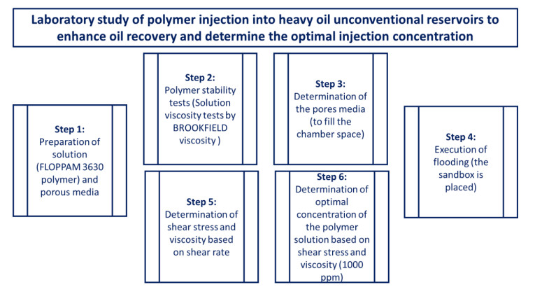
Polymers have been used for many years to control the mobility of injected water and increase the rate of oil extraction from unconventional reservoirs. Polymer flossing improves the volume of the broom, reduces the finger effect, creates channels, and delays water breakage. The combination of these processes has the potential to increase oil production and reduce production costs. To carry out this process, various polymers are used alone or in combination with surfactants and alkalis. In this study, a new type of polymer called FLOPPAM 3630 has been used to investigate the overload of very heavy oil reservoirs. For this purpose, six polymer solutions with different concentrations were made, and stability tests on shear rate, time, and temperature were performed. The polymer's stability results indicate that it is stable under other shear rate, temperature, and time passage conditions. As a result, this polymer is a suitable candidate for conducting silicification tests in reservoir temperature conditions. Then three more suitable polymer solutions were selected, and the polymer was polished. The results showed that the solution with a concentration of 1000 ppm has the best yield of about 40%. The reason for the good efficiency of this concentration is that the surface and vertical sweepers are higher than the other concentrations. Also, the difference in efficiency between less than 1000 and 2000 ppm is greater because it is more economical, and its injectability is easier to use with less concentration. Furthermore, the oil efficiency of this type of polymer in sandblasting is higher than that of other polymers tested under these conditions, making its use more economical.

| [1] |
Ning S, Barnes J, Edwards R, et al. (2019) First Ever Polymer Flood Field Pilot to Enhance the Recovery of Heavy Oils on Alaska's North Slope—Polymer Injection Performance. URTeC Soc Explor Geophys, 1671–1688. https://doi.org/10.15530/urtec-2019-643 doi: 10.15530/urtec-2019-643

|
| [2] |
Rellegadla S, Prajapat G, Agrawal A (2017) Polymers for enhanced oil recovery: fundamentals and selection criteria. Appl Microbiol Biotechnol 101: 4387–4402. https://doi.org/10.1007/s00253-017-8307-4 doi: 10.1007/s00253-017-8307-4
|
| [3] |
Farzaneh SA, Sohrabi M (2013) A review of the status of foam applications in enhanced oil recovery. EAGE Ann Conf Exhib. https://doi.org/10.2118/164917-MS doi: 10.2118/164917-MS
|
| [4] |
Ebadati A, Akbari E, Davarpanah A (2019) An experimental study of alternative hot water alternating gas injection in a fractured model. Energy Explor Exploit 37: 945–959. https://doi.org/10.1177/0144598718815247 doi: 10.1177/0144598718815247
|
| [5] |
ShamsiJazeyi H, Miller CA, Wong MS, et al. (2014) Polymer‐coated nanoparticles for enhanced oil recovery. J Appl Polym Sci 131. https://doi.org/10.1002/app.40576 doi: 10.1002/app.40576
|
| [6] |
Al-Anssari S, Ali M, Alajmi M, et al. (2021) Synergistic effect of nanoparticles and polymers on the rheological properties of injection fluids: implications for enhanced oil recovery. Energy Fuels 35: 6125–6135. https://doi.org/10.1021/acs.energyfuels.1c00105 doi: 10.1021/acs.energyfuels.1c00105
|
| [7] | Syed FI, Dahaghi AK, Muther T (2022) Laboratory to field scale assessment for EOR applicability in tight oil reservoirs. Pet Sci. In press. https://doi.org/10.1016/j.petsci.2022.04.014 |
| [8] | Khlaifat A, Qutob H, Barakat N, et al. (2011) Taking up unconventional challenge is a game changer in oil and gas industry. |
| [9] | Gotawala DR, Gates ID (2009) SAGD subcool control with smart injection wells. EUROPEC/EAGE Conf Exhib. |
| [10] | Neil JD, Chang HL, Geffen TM (1983) Waterflooding and improved waterflooding. Improved Oil Recovery. |
| [11] |
Cheraghian G, Hendraningrat L (2016) A review on applications of nanotechnology in the enhanced oil recovery part A: effects of nanoparticles on interfacial tension. Int Nano Lett 6: 129–138. https://doi.org/10.1007/s40089-015-0173-4 doi: 10.1007/s40089-015-0173-4
|
| [12] |
Taber JJ, Martin FD, Seright RS (1997) EOR screening criteria revisited-Part 1: Introduction to screening criteria and enhanced recovery field projects. SPE Res Eng 12: 189–198. https://doi.org/10.2118/35385-PA doi: 10.2118/35385-PA
|
| [13] |
Taber JJ, Martin FD, Seright RS (1997) EOR screening criteria revisited—part 2: applications and impact of oil prices. SPE Res Eng 12: 199–206. https://doi.org/10.2118/39234-PA doi: 10.2118/39234-PA
|
| [14] |
Kumar M, Hoang V, Satik C, et al. (2008) High-mobility-ratio waterflood performance prediction: challenges and new insights. SPE Res Eval Eng 11: 186–196. https://doi.org/10.2118/97671-PA doi: 10.2118/97671-PA
|
| [15] |
Rajabi M, Beheshtian S, Davoodi S, et al. (2021) Novel hybrid machine learning optimizer algorithms to prediction of fracture density by petrophysical data. J Petrol Explor Prod Technol 11: 4375–4397. https://doi.org/10.1007/s13202-021-01321-z doi: 10.1007/s13202-021-01321-z
|
| [16] |
Rajabi M, Ghorbani H, Lajmorak S (2022) Comparison of artificial intelligence algorithms to predict pore pressure using petrophysical log data. J Struct Const Eng. https://doi.org/10.22065/JSCE.2022.309523.2600 doi: 10.22065/JSCE.2022.309523.2600
|
| [17] |
Rashidi S, Mehrad M, Ghorbani H, et al. (2021) Determination of bubble point pressure & oil formation volume factor of crude oils applying multiple hidden layers extreme learning machine algorithms. J Struct Const Eng 202: 108425. https://doi.org/10.1016/j.petrol.2021.108425 doi: 10.1016/j.petrol.2021.108425
|
| [18] |
Rashidi S, Mohamadian N, Ghorbani H, et al. (2020) Shear modulus prediction of embedded pressurized salt layers and pinpointing zones at risk of casing collapse in oil and gas wells. J Appl Geophys 183: 104205. https://doi.org/10.1016/j.jappgeo.2020.104205 doi: 10.1016/j.jappgeo.2020.104205
|
| [19] |
Puskas S, Vago A, Toro M, et al. (2018) Surfactant-polymer EOR from laboratory to the pilot. SPE EOR Conf. https://doi.org/10.2118/190369-MS doi: 10.2118/190369-MS
|
| [20] |
Delamaide E, Bazin B, Rousseau D, et al. (2014) Chemical EOR for heavy oil: The Canadian experience. SPE EOR Conf. https://doi.org/10.2118/169715-MS doi: 10.2118/169715-MS
|
| [21] |
Delamaide E, Tabary R, Rousseau D (2014) Chemical EOR in low permeability reservoirs. SPE EOR Conf. https://doi.org/10.2118/169673-MS doi: 10.2118/169673-MS
|
| [22] |
Syed FI, Muther T, Van VP, et al. (2022) Numerical trend analysis for factors affecting EOR performance and CO2 storage in tight oil reservoirs. Fuel 316: 123370. https://doi.org/10.1016/j.fuel.2022.123370 doi: 10.1016/j.fuel.2022.123370
|
| [23] |
Syed FI, Muther T, Dahaghi AK, et al. (2022) CO2 EOR performance evaluation in an unconventional reservoir through mechanistic constrained proxy modeling. Fuel 310: 122390. https://doi.org/10.1016/j.fuel.2021.122390 doi: 10.1016/j.fuel.2021.122390
|
| [24] |
Muther T, Qureshi HA, Syed FI, et al. (2022) Unconventional hydrocarbon resources: geological statistics, petrophysical characterization, and field development strategies. J Petrol Explor Prod Technol 12: 1463–1488. https://doi.org/10.1007/s13202-021-01404-x doi: 10.1007/s13202-021-01404-x
|
| [25] |
Martyushev DA, Govindarajan SK (2021) Development and study of a visco-elastic gel with controlled destruction times for killing oil wells. J King Saud Univ Eng Sci. https://doi.org/10.1016/j.jksues.2021.06.007 doi: 10.1016/j.jksues.2021.06.007
|
| [26] |
Martyushev DA, Govindarajan SK, Li Y, et al. (2022) Experimental study of the influence of the content of calcite and dolomite in the rock on the efficiency of acid treatment. J Pet Sci Eng 208: 109770. https://doi.org/10.1016/j.petrol.2021.109770 doi: 10.1016/j.petrol.2021.109770
|
| [27] |
Martyushev DA, Ponomareva IN, Galkin Ⅵ (2021) Conditions for Effective Application of the Decline Curve Analysis Method. Energies 14: 6461. https://doi.org/10.3390/en14206461 doi: 10.3390/en14206461
|
| [28] |
Martyushev DA, Yurikov A (2021) Evaluation of opening of fractures in the Logovskoye carbonate reservoir, Perm Krai, Russia. Pet Res 6: 137–143. https://doi.org/10.1016/j.ptlrs.2020.11.002 doi: 10.1016/j.ptlrs.2020.11.002
|
| [29] | Terry RE, Rogers JB, Craft BC (2015) Applied petroleum reservoir engineering, Pearson Education. |
| [30] |
Gao CH (2011) Advances of polymer flood in heavy oil recovery. SPE Heavy Oil Conf Exhib. https://doi.org/10.2118/150384-MS doi: 10.2118/150384-MS
|
| [31] |
Al-Bahar MA, Merrill R, Peake W, et al. (2004) Evaluation of IOR potential within Kuwait. Abu Dhabi Int Conf Exhib. https://doi.org/10.2118/88716-MS doi: 10.2118/88716-MS
|
| [32] |
Souraki Y, Ashrafi M, Karimaie H, et al. (2012) Experimental analyses of Athabasca bitumen properties and field scale numerical simulation study of effective parameters on SAGD performance. Energy Environ Res 2: 140. https://doi.org/10.5539/eer.v2n1p140 doi: 10.5539/eer.v2n1p140
|
| [33] |
Corredor LM, Husein MM, Maini BB (2019) Effect of hydrophobic and hydrophilic metal oxide nanoparticles on the performance of xanthan gum solutions for heavy oil recovery. Nanomaterials 9: 94. https://doi.org/10.3390/nano9010094 doi: 10.3390/nano9010094
|
| [34] |
Mohamadian N, Ghorbani H, Bazrkar H, et al. (2022) Carbon-nanotube-polymer nanocomposites enable wellbore cements to better inhibit gas migration and enhance sustainability of natural gas reservoirs. Sustainable Nat Gas Reservoir Prod Eng 243–268. https://doi.org/10.1016/B978-0-12-824495-1.00005-X doi: 10.1016/B978-0-12-824495-1.00005-X
|
| [35] |
Mohamadian N, Ghorbani H, Wood DA, et al. (2018) Rheological and filtration characteristics of drilling fluids enhanced by nanoparticles with selected additives: an experimental study. Adv Geo-Energy Res 2: 228–236. https://doi.org/10.26804/ager.2018.03.01 doi: 10.26804/ager.2018.03.01
|
| [36] |
Mohamadian N, Ghorbani H, Wood DA, et al. (2019) A hybrid nanocomposite of poly (styrene-methyl methacrylate-acrylic acid)/clay as a novel rheology-improvement additive for drilling fluids. J Polym Res 26: 33. https://doi.org/10.1007/s10965-019-1696-6 doi: 10.1007/s10965-019-1696-6
|
| [37] |
Wang J, Dong M (2007) A laboratory study of polymer flooding for improving heavy oil recovery. Can Int Pet Conf. https://doi.org/10.2118/2007-178 doi: 10.2118/2007-178
|
| [38] | Khodaeipour M, Moqadam DL, Dashtbozorg A, et al. (2018) Nano Clay Effect on Adsorption of Benzene, Toluene and Xylene from Aqueous Solution. Am J Oil Chem Technol. |
| [39] | Kohlruss D, Pedersen PK, Chi G (2012) Structure and isopach mapping of the Lower Cretaceous Dina Member of the Mannville Group of northwestern Saskatchewan. Summ Inves 1: 2012–2014. |
| [40] |
Komery DP, Luhning RW, O'Rourke JG (1999) Towards commercialization of the UTF project using surface drilled horizontal SAGD wells. J Can Pet Technol 38: 36–43. https://doi.org/10.2118/99-09-03 doi: 10.2118/99-09-03
|
| [41] | Lake LW (1989) Enhanced oil recovery, United States. |
| [42] |
Liu C, Zhang L, Li Y, et al. (2022) Effects of microfractures on permeability in carbonate rocks based on digital core technology. Adv Geo-Energy Res 6: 86–90. https://doi.org/10.46690/ager.2022.01.07 doi: 10.46690/ager.2022.01.07
|
| [43] |
Martyushev DA (2020) Modeling and prediction of asphaltene-resin-paraffinic substances deposits in oil production wells. Georesursy 22: 86–92. https://doi.org/10.18599/grs.2020.4.86-92 doi: 10.18599/grs.2020.4.86-92
|


Figures(9) / Tables(3)

Pezhman Soltani Tehrani, Hamzeh Ghorbani, Sahar Lajmorak, Omid Molaei, Ahmed E Radwan, Saeed Parvizi Ghaleh. Laboratory study of polymer injection into heavy oil unconventional reservoirs to enhance oil recovery and determination of optimal injection concentration[J]. AIMS Geosciences, 2022, 8(4): 579-592. doi: 10.3934/geosci.2022031


 DownLoad: