SSMM-DS: A semantic segmentation model for mangroves based on Deeplabv3+ with swin transformer

Zhenhua Wang; Jinlong Yang; Chuansheng Dong; Xi Zhang; Congqin Yi; Jiuhu Sun; Zhenhua Wang; Jinlong Yang; Chuansheng Dong; Xi Zhang; Congqin Yi; Jiuhu Sun

doi:10.3934/era.2024260

Electronic Research Archive

2024, Volume 32, Issue 10: 5615-5632. doi: 10.3934/era.2024260

Previous Article Next Article

Research article Special Issues

SSMM-DS: A semantic segmentation model for mangroves based on Deeplabv3+ with swin transformer

1.
College of Information Technology, Shanghai Ocean University, Shanghai 201306, China
2.
Shandong Land Surveying and Mapping Institute, Jinan 250000, China
3.
Shandong provincial institute of land space data and remote sensing technology, Jinan 250000, China

Received: 21 July 2024 Revised: 06 September 2024 Accepted: 23 September 2024 Published: 15 October 2024

Mangrove wetlands play a crucial role in maintaining species diversity. However, they face threats from habitat degradation, deforestation, pollution, and climate change. Detecting changes in mangrove wetlands is essential for understanding their ecological implications, but it remains a challenging task. In this study, we propose a semantic segmentation model for mangroves based on Deeplabv3+ with Swin Transformer, abbreviated as SSMM-DS. Using Deeplabv3+ as the basic framework, we first constructed a data concatenation module to improve the contrast between mangroves and other vegetation or water. We then employed Swin Transformer as the backbone network, enhancing the capability of global information learning and detail feature extraction. Finally, we optimized the loss function by combining cross-entropy loss and dice loss, addressing the issue of sampling imbalance caused by the small areas of mangroves. Using GF-1 and GF-6 images, taking mean precision (mPrecision), mean intersection over union (mIoU), floating-point operations (FLOPs), and the number of parameters (Params) as evaluation metrics, we evaluate SSMM-DS against state-of-the-art models, including FCN, PSPNet, OCRNet, uPerNet, and SegFormer. The results demonstrate SSMM-DS's superiority in terms of mIoU, mPrecision, and parameter efficiency. SSMM-DS achieves a higher mIoU (95.11%) and mPrecision (97.79%) while using fewer parameters (17.48M) compared to others. Although its FLOPs are slightly higher than SegFormer's (15.11G vs. 9.9G), SSMM-DS offers a balance between performance and efficiency. Experimental results highlight SSMM-DS's effectiveness in extracting mangrove features, making it a valuable tool for monitoring and managing these critical ecosystems.
- remote sensing image,
- semantic segmentation,
- mangrove,
- swin transformer
Citation: Zhenhua Wang, Jinlong Yang, Chuansheng Dong, Xi Zhang, Congqin Yi, Jiuhu Sun. SSMM-DS: A semantic segmentation model for mangroves based on Deeplabv3+ with swin transformer[J]. Electronic Research Archive, 2024, 32(10): 5615-5632. doi: 10.3934/era.2024260

Related Papers:

Abstract

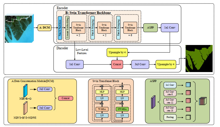
Mangrove wetlands play a crucial role in maintaining species diversity. However, they face threats from habitat degradation, deforestation, pollution, and climate change. Detecting changes in mangrove wetlands is essential for understanding their ecological implications, but it remains a challenging task. In this study, we propose a semantic segmentation model for mangroves based on Deeplabv3+ with Swin Transformer, abbreviated as SSMM-DS. Using Deeplabv3+ as the basic framework, we first constructed a data concatenation module to improve the contrast between mangroves and other vegetation or water. We then employed Swin Transformer as the backbone network, enhancing the capability of global information learning and detail feature extraction. Finally, we optimized the loss function by combining cross-entropy loss and dice loss, addressing the issue of sampling imbalance caused by the small areas of mangroves. Using GF-1 and GF-6 images, taking mean precision (mPrecision), mean intersection over union (mIoU), floating-point operations (FLOPs), and the number of parameters (Params) as evaluation metrics, we evaluate SSMM-DS against state-of-the-art models, including FCN, PSPNet, OCRNet, uPerNet, and SegFormer. The results demonstrate SSMM-DS's superiority in terms of mIoU, mPrecision, and parameter efficiency. SSMM-DS achieves a higher mIoU (95.11%) and mPrecision (97.79%) while using fewer parameters (17.48M) compared to others. Although its FLOPs are slightly higher than SegFormer's (15.11G vs. 9.9G), SSMM-DS offers a balance between performance and efficiency. Experimental results highlight SSMM-DS's effectiveness in extracting mangrove features, making it a valuable tool for monitoring and managing these critical ecosystems.

References

[1]	N. C. Duke, J. Meynecke, S. Dittmann, A. M. Ellison, K. Anger, U. Berger, et al., A world without mangroves?, Science, 317 (2007), 41–42. https://doi.org/10.1126/science.317.5834.41b doi: 10.1126/science.317.5834.41b
[2]	P. L. Biswas, S. R. Biswas, Mangrove forests: Ecology, management, and threats, Life Land, (2019), 1–14. https://doi.org/10.1007/978-3-319-71065-5_26-1 doi: 10.1007/978-3-319-71065-5_26-1
[3]	C. Giri, Frontiers in global mangrove forest monitoring, Remote Sens., 15 (2023), 3852. https://doi.org/10.3390/rs15153852 doi: 10.3390/rs15153852
[4]	S. C. Basha, An overview on global mangroves distribution, Indian J. Geo Mar. Sci., 47 (2018), 766–772.
[5]	Y. Sun, D. Zhao, W. Guo, Y. Gao, X. Su, B. Wei, A review on the application of remote sensing in mangrove ecosystem monitoring, Acta Ecol. Sin., 33 (2013), 4523–4538. https://doi.org/10.5846/stxb201205150715 doi: 10.5846/stxb201205150715
[6]	R. Vidhya, D. Vijayasekaran, M. Ahamed Farook, S. Jai, M. Rohini, A. Sinduja, Improved Classification of mangroves health status using hyperspectral remote sensing data, Int. Arch. Photogramm. Remote Sens. Spat. Inf. Sci., 8 (2014), 667–670. https://doi.org/10.5194/isprsarchives-XL-8-667-2014 doi: 10.5194/isprsarchives-XL-8-667-2014
[7]	T. D. Pham, D. T. Bui, K. Yoshino, N. N. Le, Optimized rule-based logistic model tree algorithm for mapping mangrove species using ALOS PALSAR imagery and GIS in the tropical region, Environ. Earth Sci., 77 (2018), 159. https://doi.org/10.1007/s12665-018-7373-y doi: 10.1007/s12665-018-7373-y
[8]	L. Li, W. Liu, Y. Tao, X. Xu, W. Fu, J. Dong, Diffusion dynamics and driving forces of Spartina alterniflora in the Guangxi Shankou Mangrove Reserve, Acta Ecol. Sin., 41 (2021), 6814–6824.
[9]	J. Cao, K. Liu, L. Zhuo, L. Liu, Y. Zhu, L. Peng, Combining UAV-based hyperspectral and LiDAR data for mangrove species classification using the rotation forest algorithm, Int. J. Appl. Earth Obs. Geoinformation, 102 (2021), 102414. https://doi.org/10.1016/j.jag.2021.102414 doi: 10.1016/j.jag.2021.102414
[10]	M. Di Cicco, C. Potena, G. Grisetti, A. Pretto, Automatic model based dataset generation for fast and accurate crop and weeds detection, in 2017 IEEE/RSJ International Conference on Intelligent Robots and Systems (IROS), (2017), 5188–5195. https://doi.org/10.1109/IROS.2017.8206408
[11]	D. Lee, C. Kim, S. Kim, M. Cho, W. Han, Autoregressive image generation using residual quantization, in 2022 IEEE/CVF Conference on Computer Vision and Pattern Recognition (CVPR), (2022), 11513–11522. https://doi.org/10.1109/CVPR52688.2022.01123
[12]	L. Wang, R. Li, C. Zhang, S. Fang, C. Duan, X. Meng, et al., UNetFormer: A UNet-like transformer for efficient semantic segmentation of remote sensing urban scene imagery, ISPRS J. Photogramm. Remote Sens., 190 (2022), 196–214. https://doi.org/10.1016/j.isprsjprs.2022.06.008 doi: 10.1016/j.isprsjprs.2022.06.008
[13]	X. Yuan, J. Shi, L. Gu, A review of deep learning methods for semantic segmentation of remote sensing imagery, Expert Syst. Appl., 169 (2021), 114417. https://doi.org/10.1016/j.eswa.2020.114417 doi: 10.1016/j.eswa.2020.114417
[14]	A. A. Aleissaee, A. Kumar, R. M. Anwer, S. Khan, H. Cholakkal, G. Xia, et al., Transformers in Remote Sensing: A Survey, Remote Sens., 15 (2023), 1860. https://doi.org/10.3390/rs15071860 doi: 10.3390/rs15071860
[15]	L. Wan, H. Zhang, G. Lin, H. Lin, A small-patched convolutional neural network for mangrove mapping at species level using high-resolution remote-sensing image, Ann. GIS, 25 (2019), 45–55. https://doi.org/10.1080/19475683.2018.1564791 doi: 10.1080/19475683.2018.1564791
[16]	G. M. D. S. Moreno, O. A. D. Carvalho Júnior, O. L. F. D. Carvalho, T. C. Andrade, Deep semantic segmentation of mangroves in Brazil combining spatial, temporal, and polarization data from Sentinel-1 time series, Ocean Coastal Manage., 231 (2023), 106381. https://doi.org/10.1016/j.ocecoaman.2022.106381 doi: 10.1016/j.ocecoaman.2022.106381
[17]	Y. Fan, Q. Zeng, Z. Mei, W. Hu, Semantic segmentation for mangrove using spectral indices and self-attention mechanism, in 2022 7th International Conference on Signal and Image Processing (ICSIP), (2022), 436–441. https://doi.org/10.1109/ICSIP55141.2022.9886553
[18]	C. Xu, J. Wang, Y. Sang, K. Li, J. Liu, G. Yang, An effective deep learning model for monitoring mangroves: A case study of the Indus Delta, Remote Sens., 15 (2023), 2220. https://doi.org/10.3390/rs15092220 doi: 10.3390/rs15092220
[19]	C. Kuenzer, A. Bluemel, S. Gebhardt, T. V. Quoc, S. Dech, Remote sensing of mangrove ecosystems: A Review, Remote Sens., 3 (2011), 878–928. https://doi.org/10.3390/rs3050878 doi: 10.3390/rs3050878
[20]	K. Maurya, S. Mahajan, N. Chaube, Remote sensing techniques: mapping and monitoring of mangrove ecosystem-A review, Complex Intell. Syst., 7 (2021), 2797–2818. https://doi.org/10.1007/s40747-021-00457-z doi: 10.1007/s40747-021-00457-z
[21]	C. Giri, Observation and monitoring of mangrove forests using remote sensing: Opportunities and challenges, Remote Sens., 8 (2016), 783. https://doi.org/10.3390/rs8090783 doi: 10.3390/rs8090783
[22]	T. V. Tran, R. Reef, X. Zhu, A review of spectral indices for mangrove remote sensing, Remote Sens., 14 (2022), 4868. https://doi.org/10.3390/rs14194868 doi: 10.3390/rs14194868
[23]	C. Liu, P. Sun, S. Liu, A review of plant spectral reflectance response to water physiological changes, Chin. J. Plant Ecol., 40 (2016), 80–91. https://doi.org/10.17521/cjpe.2015.0267 doi: 10.17521/cjpe.2015.0267
[24]	J. Xue, B. Su, Significant remote sensing vegetation indices: A review of developments and applications, J. Sens., (2017). https://doi.org/10.1155/2017/1353691 doi: 10.1155/2017/1353691
[25]	B. Gao, NDWI-A normalized difference water index for remote sensing of vegetation liquid water from space, Remote Sens. Environ., 58 (1996), 257–266. https://doi.org/10.1016/S0034-4257(96)00067-3 doi: 10.1016/S0034-4257(96)00067-3
[26]	K. He, X. Zhang, S. Ren, J. Sun, Deep residual learning for image recognition, in 2016 IEEE Conference on Computer Vision and Pattern Recognition (CVPR), (2016), 770–778. https://doi.org/10.1109/CVPR.2016.90
[27]	A. Vaswani, N. Shazeer, N. Parmar, J. Uszkoreit, L. Jones, A. N. Gomez, et al., Attention is all you need, in Proceedings of the 31st International Conference on Neural Information Processing Systems, (2017), 6000–6010.
[28]	X. Li, X. Sun, Y. Meng, J. Liang, F. Wu, J. Li, Dice loss for data-imbalanced NLP tasks, in Proceedings of the 58th Annual Meeting of the Association for Computational Linguistics, (2020), 465–476. https://doi.org/10.18653/v1/2020.acl-main.45
[29]	L. Chen, Y. Zhu, G. Papandreou, F. Schroff, H. Adam, Encoder-decoder with atrous separable convolution for semantic image segmentation, in Computer Vision-ECCV 2018, 11211 (2018), 833–851. https://doi.org/10.1007/978-3-030-01234-2_49
[30]	C. Shorten, T. M. Khoshgoftaar, A survey on image data augmentation for deep learning, J. Big Data, 6 (2019). https://doi.org/10.1186/s40537-019-0197-0 doi: 10.1186/s40537-019-0197-0
[31]	J. Long, E. Shelhamer, T. Darrell, Fully convolutional networks for semantic segmentation, in 2015 IEEE Conference on Computer Vision and Pattern Recognition (CVPR), (2015), 3431–3440. https://doi.org/10.1109/CVPR.2015.7298965
[32]	H. Zhao, J. Shi, X. Qi, X. Wang, J. Jia, Pyramid scene parsing network, in 2017 IEEE Conference on Computer Vision and Pattern Recognition (CVPR), (2017), 6230–6239. https://doi.org/10.1109/CVPR.2017.660
[33]	Y. Yuan, X. Chen, J. Wang, Object-contextual representations for semantic segmentation, in Computer vision-ECCV 2020, 12351 (2020), 173–190. https://doi.org/10.1007/978-3-030-58539-6_11
[34]	T. Xiao, Y. Liu, B. Zhou, Y. Jiang, J. Sun, Unified perceptual parsing for scene understanding, in Computer Vision-ECCV 2018: 15th European Conference, (2018), 432–448. https://doi.org/10.1007/978-3-030-01228-1_26
[35]	E. Xie, W. Wang, Z. Yu, A. Anandkumar, J. M. Alvarez, P. Luo, SegFormer: Simple and efficient design for semantic segmentation with transformers, in Proceedings of the 35th International Conference on Neural Information Processing Systems, 34 (2021), 12077–12090.

Reader Comments

Your name:*

Email:*
© 2024 the Author(s), licensee AIMS Press. This is an open access article distributed under the terms of the Creative Commons Attribution License (http://creativecommons.org/licenses/by/4.0)