Second-order general Emden-Fowler differential equations of neutral type: Improved Kamenev-type oscillation criteria

Asma Al-Jaser; Osama Moaaz; Asma Al-Jaser; Osama Moaaz

doi:10.3934/era.2024241

Electronic Research Archive

2024, Volume 32, Issue 9: 5231-5248. doi: 10.3934/era.2024241

Previous Article Next Article

Research article

Second-order general Emden-Fowler differential equations of neutral type: Improved Kamenev-type oscillation criteria

Asma Al-Jaser ^{1
,
,},
Osama Moaaz ^{2
,
,}

1.
Department of Mathematical Sciences, College of Science, Princess Nourah bint Abdulrahman University, P.O. Box 84428, Riyadh 11671, Saudi Arabia
2.
Department of Mathematics, College of Science, Qassim University, P.O. Box 6644, Buraydah 51452, Saudi Arabia

Received: 10 July 2024 Revised: 07 August 2024 Accepted: 28 August 2024 Published: 09 September 2024

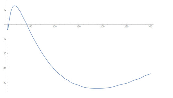
The study of the oscillatory behavior of a general class of neutral Emden-Fowler differential equations is the focus of this work. The main motivations for studying the oscillatory behavior of neutral equations are their many applications as well as the richness of these equations with exciting analytical issues. We obtained novel oscillation conditions in Kamenev-type criteria for the considered equation in the canonical case. We improve the monotonic and asymptotic characteristics of the non-oscillatory solutions to the considered equation and then utilize these characteristics to refine the oscillation conditions. We present, through examples and discussions, what demonstrates the novelty and efficiency of the results compared to previous relevant findings in the literature. In addition, we numerically represent the solutions of some special cases to support the theoretical results.
- differential equations,
- Kamenev-type criteria,
- oscillation theory,
- canonical case,
- neutral argument
Citation: Asma Al-Jaser, Osama Moaaz. Second-order general Emden-Fowler differential equations of neutral type: Improved Kamenev-type oscillation criteria[J]. Electronic Research Archive, 2024, 32(9): 5231-5248. doi: 10.3934/era.2024241

Related Papers:

Abstract

The study of the oscillatory behavior of a general class of neutral Emden-Fowler differential equations is the focus of this work. The main motivations for studying the oscillatory behavior of neutral equations are their many applications as well as the richness of these equations with exciting analytical issues. We obtained novel oscillation conditions in Kamenev-type criteria for the considered equation in the canonical case. We improve the monotonic and asymptotic characteristics of the non-oscillatory solutions to the considered equation and then utilize these characteristics to refine the oscillation conditions. We present, through examples and discussions, what demonstrates the novelty and efficiency of the results compared to previous relevant findings in the literature. In addition, we numerically represent the solutions of some special cases to support the theoretical results.

References

[1]	A. Ghezal, M. Balegh, I. Zemmouri, Solutions and local stability of the Jacobsthal system of difference equations, AIMS Math., 9 (2024), 3576–3591. https://doi.org/10.3934/math.2024175 doi: 10.3934/math.2024175
[2]	M. M. Alam, M. Arshad, F. M. Alharbi, A. Hassan, Q. Haider, L. A. Al-Essa, et al., Comparative dynamics of mixed convection heat transfer under thermal radiation effect with porous medium flow over dual stretched surface, Sci. Rep., 13 (2023). https://doi.org/10.1038/s41598-023-40040-9 doi: 10.1038/s41598-023-40040-9
[3]	A. M. Saeed, S. H. Alotaibi, Numerical methods for solving the home heating system, Adv. Dyn. Syst. Appl., 17 (2020), 581–598.
[4]	A. Maneengam, S. E. Ahmed, A. M. Saeed, A. Abderrahmane, O. Younis, K. Guedri, et al., Numerical study of heat transfer enhancement within confined shell and tube latent heat thermal storage microsystem using hexagonal PCMs, Micromachines, 13 (2022), 1062. https://doi.org/10.3390/mi13071062 doi: 10.3390/mi13071062
[5]	V. Volterra, Sur la théorie mathématique des phénomènes héréditaires, J. Math. Pures Appl., 7 (1928), 249–298.
[6]	A. D. Mishkis, Lineare Differentialgleichungen Mit Nacheilendem Argument, Deutscher Verlag der Wissenschaften, 1955.
[7]	R. Bellman, J. M. Danskin, A Survey of the Mathematical Theory of Time-Lag, Retarded Control, and Hereditary Processes, RAND Corporation, Santa Monica, CA, 1954.
[8]	R. Bellman, K. L. Cooke, R. Bellman, J. Gillis, Differential difference equations, Phys. Today, 16 (1963), 75–76. https://doi.org/10.1063/1.3050672 doi: 10.1063/1.3050672
[9]	R. P. Agarwal, S. R. Grace, D. O'Regan, Oscillation Theory for Difference and Functional Differential Equations, Kluwer Academic, 2000. https://doi.org/10.1007/978-94-015-9401-1
[10]	R. P. Agarwal, S. R. Grace, D. O'Regan, Oscillation Theory for Second Order Linear, Half-Linear, Superlinear and Sublinear Dynamic Equations, Kluwer Academic Publishers, Dordrecht, 2002. https://doi.org/10.1007/978-94-015-9401-1
[11]	R. P. Agarwal, M. Bohner, W. T. Li, Nonoscillation and oscillation: Theory for functional differential equations, in Monographs and Textbooks in Pure and Applied Mathematics, Marcel Dekker, Inc., New York, 267 (2004). https://doi.org/10.1201/9780203025741
[12]	I. Gyori, G. Ladas, Oscillation Theory of Delay Differential Equations with Applications, Clarendon Press, Oxford, 1991. https://doi.org/10.1093/oso/9780198535829.001.0001
[13]	L. H. Erbe, Q. Kong, B. G. Zhong, Oscillation Theory for Functional Differential Equations, Marcel Dekker, New York, 1995.
[14]	J. K. Hale, Functional differential equations, in Analytic Theory of Differential Equations, Springer, Berlin/Heidelberg, 1971.
[15]	J. Džurina, B. Mihalíková, Oscillation criteria for second order neutral differential equations, Math. Bohemica, 125 (2000), 145–153. https://doi.org/10.21136/mb.2000.125960 doi: 10.21136/mb.2000.125960
[16]	Z. Han, T. Li, S. Sun, W. Chen, On the oscillation of second-order neutral delay differential equations, Adv. Differ. Equations, 2010 (2010), 1–9. https://doi.org/10.1155/2010/289340 doi: 10.1155/2010/289340
[17]	J. Džurina, Oscillation theorems for second order advanced neutral differential equations, Tatra Mt. Math. Publ., 48 (2011), 61–71. https://doi.org/10.2478/v10127-011-0006-4 doi: 10.2478/v10127-011-0006-4
[18]	Y. Şahiner, On oscillation of second order neutral type delay differential equations, Appl. Math. Comput., 150 (2004), 697–706. https://doi.org/10.1016/s0096-3003(03)00300-x doi: 10.1016/s0096-3003(03)00300-x
[19]	O. Moaaz, A. Muhib, S. Owyed, E. E. Mahmoud, A. Abdelnaser, Second-order neutral differential equations: Improved criteria for testing the oscillation, J. Math., 2021 (2021), 1–7. https://doi.org/10.1155/2021/6665103 doi: 10.1155/2021/6665103
[20]	T. Hassan, O. Moaaz, A. Nabih, M. Mesmouli, A. El-Sayed, New sufficient conditions for oscillation of second-order neutral delay differential equations, Axioms, 10 (2021), 281. https://doi.org/10.3390/axioms10040281 doi: 10.3390/axioms10040281
[21]	O. Moaaz, C. Cesarano, B. Almarri, An improved relationship between the solution and its corresponding function in fourth-order neutral differential equations and its applications, Mathematics, 11 (2023), 1708. https://doi.org/10.3390/math11071708 doi: 10.3390/math11071708
[22]	Q. Feng, B. Zheng, Oscillation criteria for nonlinear third-order delay dynamic equations on time scales involving a super-linear neutral term, Fractal Fractional, 8 (2024), 115. https://doi.org/10.3390/fractalfract8020115 doi: 10.3390/fractalfract8020115
[23]	K. S. Vidhyaa, R. Deepalakshmi, J. Graef, E. Thandapani, Oscillatory behavior of semi-canonical third-order delay differental equations with a superlinear neutral term, Appl. Anal. Discrete Math., 2024 (2024), 6. https://doi.org/10.2298/aadm210812006v doi: 10.2298/aadm210812006v
[24]	N. Prabaharan, E. Thandapani, E. Tunç, Asymptotic behavior of semi-canonical third-order delay differential equations with a superlinear neutral term, Palest. J. Math., 1 (2023). https://doi.org/10.58997/ejde.2023.45 doi: 10.58997/ejde.2023.45
[25]	L. Liu, Y. Bai, New oscillation criteria for second-order nonlinear neutral delay differential equations, J. Comput. Appl. Math., 231 (2009), 657–663. https://doi.org/10.1016/j.cam.2009.04.009 doi: 10.1016/j.cam.2009.04.009
[26]	S. R. Grace, J. Džurina, I. Jadlovská, T. Li, An improved approach for studying oscillation of second-order neutral delay differential equations, J. Inequalities Appl., 2018 (2018). https://doi.org/10.1186/s13660-018-1767-y doi: 10.1186/s13660-018-1767-y
[27]	I. Jadlovská, New criteria for sharp oscillation of second-order neutral delay differential equations, Mathematics, 9 (2021), 2089. https://doi.org/10.3390/math9172089 doi: 10.3390/math9172089
[28]	I. Jadlovská, J. Džurina, Kneser-type oscillation criteria for second-order half-linear delay differential equations, Appl. Math. Comput., 380 (2020), 125289. https://doi.org/10.1016/j.amc.2020.125289 doi: 10.1016/j.amc.2020.125289
[29]	O. Moaaz, H. Ramos, J. Awrejcewicz, Second-order Emden–Fowler neutral differential equations: A new precise criterion for oscillation, Appl. Math. Lett., 118 (2021), 107172. https://doi.org/10.1016/j.aml.2021.107172 doi: 10.1016/j.aml.2021.107172
[30]	O. Moaaz, W. Albalawi, Differential equations of the neutral delay type: More efficient conditions for oscillation, AIMS Math., 8 (2023), 12729–12750. https://doi.org/10.3934/math.2023641 doi: 10.3934/math.2023641

Reader Comments

Your name:*

Email:*
© 2024 the Author(s), licensee AIMS Press. This is an open access article distributed under the terms of the Creative Commons Attribution License (http://creativecommons.org/licenses/by/4.0)