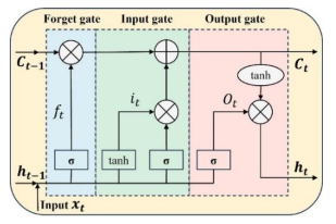
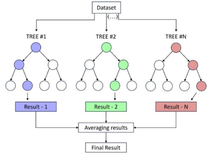
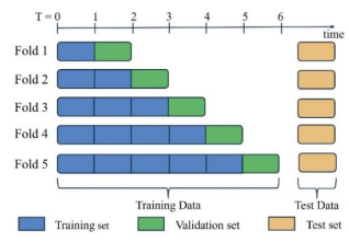
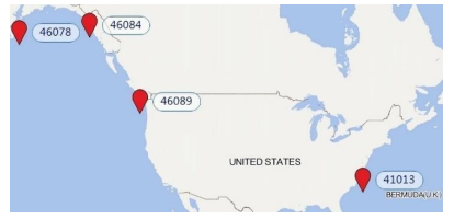
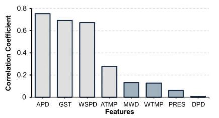
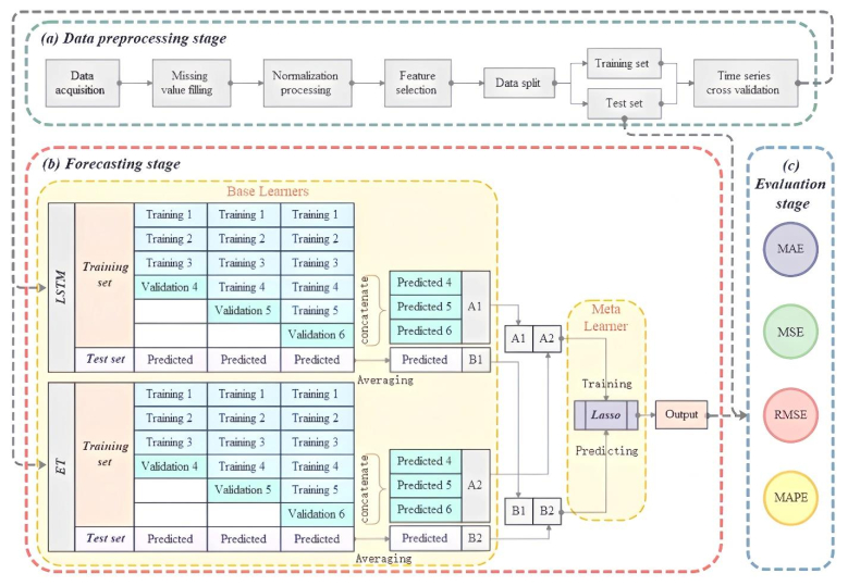
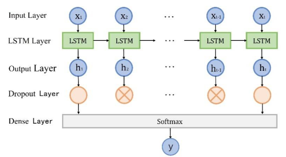
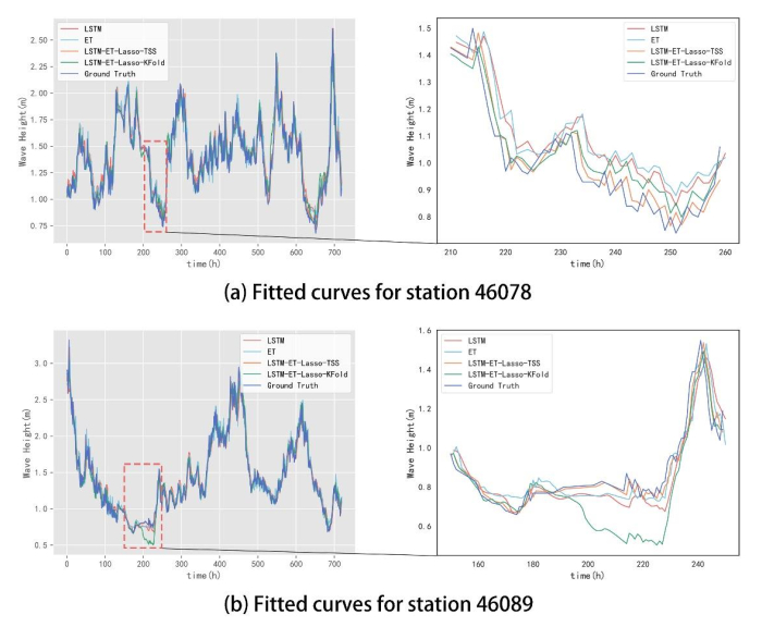
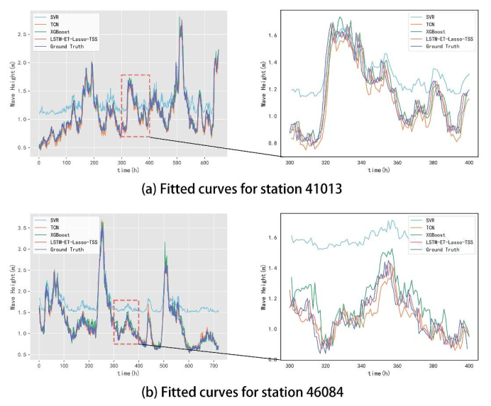
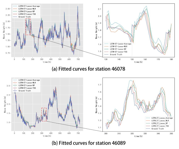
Wave height prediction is hampered by the volatility and unpredictability of ocean data. Traditional single predictors are inadequate in capturing this complexity, and weighted fusion methods fail to consider inter-model correlations, resulting in suboptimal performance. To overcome these challenges, we presented an improved stacking-based model that combined the long short-term memory (LSTM) network with extremely randomized trees (ET) for wave height prediction. Initially, features with weak correlation to wave height were excluded using the Pearson correlation coefficient. Subsequently, a stacking ensemble tailored for time series cross-validation was deployed, employing LSTM and ET as base learners to capture temporal and feature-specific patterns, respectively. Lasso regression was utilized as the meta-learner, harmonizing these insights to improve accuracy by leveraging the strengths of each model across different dimensions of the data. Validation using datasets from four buoy stations demonstrated the superior predictive capability of our proposed model over single predictors such as temporal convolutional networks (TCN) and XGBoost, and fusion methods like LSTM-ET-BP.
Citation: Peng Lu, Yuze Chen, Ming Chen, Zhenhua Wang, Zongsheng Zheng, Teng Wang, Ru Kong. An improved stacking-based model for wave height prediction[J]. Electronic Research Archive, 2024, 32(7): 4543-4562. doi: 10.3934/era.2024206
Wave height prediction is hampered by the volatility and unpredictability of ocean data. Traditional single predictors are inadequate in capturing this complexity, and weighted fusion methods fail to consider inter-model correlations, resulting in suboptimal performance. To overcome these challenges, we presented an improved stacking-based model that combined the long short-term memory (LSTM) network with extremely randomized trees (ET) for wave height prediction. Initially, features with weak correlation to wave height were excluded using the Pearson correlation coefficient. Subsequently, a stacking ensemble tailored for time series cross-validation was deployed, employing LSTM and ET as base learners to capture temporal and feature-specific patterns, respectively. Lasso regression was utilized as the meta-learner, harmonizing these insights to improve accuracy by leveraging the strengths of each model across different dimensions of the data. Validation using datasets from four buoy stations demonstrated the superior predictive capability of our proposed model over single predictors such as temporal convolutional networks (TCN) and XGBoost, and fusion methods like LSTM-ET-BP.

| [1] |
S. Shamshirband, A. Mosavi, T. Rabczuk, N. Nabipour, K. Chau, Prediction of significant wave height; comparison between nested grid numerical model, and machine learning models of artificial neural networks, extreme learning and support vector machines, Eng. Appl. Comput. Fluid Mech., 14 (2020), 805–817. https://doi.org/10.1080/19942060.2020.1773932 doi: 10.1080/19942060.2020.1773932

|
| [2] |
A. Alqushaibi, S. J. Abdulkadir, H. M. Rais, Q. Al-Tash, M. G. Ragab, H. Alhussian, Enhanced weight-optimized recurrent neural networks based on sine cosine algorithm for wave height prediction, J. Mar. Sci. Eng., 9 (2021), 524. https://doi.org/10.3390/jmse9050524 doi: 10.3390/jmse9050524
|
| [3] |
J. Swain, P. A. Umesh, P. K. Bhaskaran, A. N. Balchand, Simulation of nearshore waves using boundary conditions from WAM and WWⅢ–a case study, ISH J. Hydraul. Eng., 27 (2021), 506–520. https://doi.org/10.1080/09715010.2019.1603087 doi: 10.1080/09715010.2019.1603087
|
| [4] |
P. T. D. Spanos, ARMA algorithms for ocean wave modeling, J. Energy Resour. Technol., 105 (1983), 300–309. https://doi.org/10.1115/1.3230919 doi: 10.1115/1.3230919
|
| [5] |
N. Zheng, H. Chai, Y. Ma, L. Chen, P. Chen, Hourly sea level height forecast based on GNSS-IR by using ARIMA model, Int. J. Remote Sens., 43 (2022), 3387–3411. https://doi.org/10.1080/01431161.2022.2091965 doi: 10.1080/01431161.2022.2091965
|
| [6] |
W. Hao, X. Sun, C. Wang, H. Chen, L. Huang, A hybrid EMD-LSTM model for non-stationary wave prediction in offshore China, Ocean Eng., 246 (2022), 110566. https://doi.org/10.1016/j.oceaneng.2022.110566 doi: 10.1016/j.oceaneng.2022.110566
|
| [7] |
J. V. Bjö rkqvist, O. Vä hä -Piikkiö , V. Alari, A. Kuznetsova, L. Tuomi, WAM, SWAN and WAVEWATCH Ⅲ in the Finnish archipelago—the effect of spectral performance on bulk wave parameters, J. Oper. Oceanogr., 13 (2020), 55–70. https://doi.org/10.1080/1755876X.2019.1633236 doi: 10.1080/1755876X.2019.1633236
|
| [8] |
M. Li, K. Liu, Probabilistic prediction of significant wave height using dynamic Bayesian network and information flow, Water, 12 (2020), 2075. https://doi.org/10.3390/w12082075 doi: 10.3390/w12082075
|
| [9] | S. Contardo, R. Hoeke, P. Branson, V. Hernaman, T. Pitman, Hydrodynamic modelling for nearshore predictions, CSIRO, 2020. |
| [10] |
S. Gracia, J. Olivito, J. Resano, B. Martin-del-Brio, M. de Alfonso, E. Á lvarez, Improving accuracy on wave height estimation through machine learning techniques, Ocean Eng., 236 (2021), 108699. https://doi.org/10.1016/j.oceaneng.2021.108699 doi: 10.1016/j.oceaneng.2021.108699
|
| [11] |
E. Dakar, J. M. Fernández-Jaramillo, I. Gertman, R. Mayerle, R. Goldman, An artificial neural network based system for wave height prediction, Coastal Eng. J., 65 (2023) 309–324. https://doi.org/10.1080/21664250.2023.2190002 doi: 10.1080/21664250.2023.2190002
|
| [12] |
S. Fan, N. Xiao, S. Dong, A novel model to predict significant wave height based on long short-term memory network, Ocean Eng., 205 (2020), 107298. https://doi.org/10.1016/j.oceaneng.2020.107298 doi: 10.1016/j.oceaneng.2020.107298
|
| [13] |
S. Arslan, A hybrid forecasting model using LSTM and Prophet for energy consumption with decomposition of time series data, PeerJ Comput. Sci., 8 (2022), e1001. https://doi.org/10.7717/peerj-cs.1001 doi: 10.7717/peerj-cs.1001
|
| [14] | O. Gungor, T. S. Rosing, B. Aksanli, Opelrul: Optimally weighted ensemble learner for remaining useful life prediction, in 2021 IEEE International Conference on Prognostics and Health Management (ICPHM), Detroit (Romulus), MI, USA, (2021), 1–8. https://doi.org/10.1109/icphm51084.2021.9486535 |
| [15] |
M. Murtaza, M. Sharif, M. Yasmin, M. Fayyaz, S. Kadry, M. Y. Lee, Clothes retrieval using M-AlexNet with mish function and feature selection using joint Shannon's entropy Pearson's correlation coefficient, IEEE Access, 10 (2022), 115469–115490. https://doi.org/10.1109/access.2022.3218322 doi: 10.1109/access.2022.3218322
|
| [16] |
F. Shahid, A. Zameer, M. Muneeb, Predictions for COVID-19 with deep learning models of LSTM, GRU and Bi-LSTM, Chaos, Solitons Fractals, 140 (2020), 110212. https://doi.org/10.1016/j.chaos.2020.110212 doi: 10.1016/j.chaos.2020.110212
|
| [17] |
K. Cho, Y. Kim, Improving streamflow prediction in the WRF-Hydro model with LSTM networks, J. Hydrol., 605 (2022), 127297. https://doi.org/10.1016/j.jhydrol.2021.127297 doi: 10.1016/j.jhydrol.2021.127297
|
| [18] | S. Heddam, Intelligent data analytics approaches for predicting dissolved oxygen concentration in river: Extremely randomized tree versus random forest, MLPNN and MLR, in Intelligent Data Analytics for Decision-Support Systems in Hazard Mitigation, (eds. R. C. Deo et al.), Springer, (2021), 89–107. https://doi.org/10.1007/978-981-15-5772-9_5 |
| [19] |
M. R. C. Acosta, S. Ahmed, C. E. Garcia, I. Koo, Extremely randomized trees-based scheme for stealthy cyber-attack detection in smart grid networks, IEEE Access, 8 (2020), 19921–19933. https://doi.org/10.1109/access.2020.2968934 doi: 10.1109/access.2020.2968934
|
| [20] |
T. Yang, X. Liu, L. Wang, P. Bai, J. Li, Simulating hydropower discharge using multiple decision tree methods and a dynamical model merging technique, J. Water Resour. Plann. Manage., 146 (2020), 04019072. https://doi.org/10.1061/(ASCE)WR.1943-5452.0001146 doi: 10.1061/(ASCE)WR.1943-5452.0001146
|
| [21] |
M. Gong, J. Wang, Y. Bai, B. Li, L. Zhang, Heat load prediction of residential buildings based on discrete wavelet transform and tree-based ensemble learning, J. Build. Eng., 32 (2020), 101455. https://doi.org/10.1016/j.jobe.2020.101455 doi: 10.1016/j.jobe.2020.101455
|
| [22] |
A. D. Lainder, R. D. Wolfinger, Forecasting with gradient boosted trees: Augmentation, tuning, and cross-validation strategies: Winning solution to the M5 Uncertainty competition, Int. J. Forecasting, 38 (2022), 1426–1433. https://doi.org/10.1016/j.ijforecast.2021.12.003 doi: 10.1016/j.ijforecast.2021.12.003
|
| [23] | M. Hasanov, M. Wolter, E. Glende, Time series data splitting for Short-Term load forecasting, in PESS+ PELSS 2022; Power and Energy Student Summit, Kassel, Germany, (2022), 1–6. |
| [24] |
G. Huang, Missing data filling method based on linear interpolation and lightgbm, J. Phys. Conf. Ser., 1754 (2021), 012187. https://doi.org/10.1088/1742-6596/1754/1/012187 doi: 10.1088/1742-6596/1754/1/012187
|
| [25] |
B. G. Reguero, I. J. Losada, F. J. Méndez, A recent increase in global wave power as a consequence of oceanic warming, Nat. Commun., 10 (2019), 205. https://doi.org/10.1038/s41467-018-08066-0 doi: 10.1038/s41467-018-08066-0
|
| [26] | J. Korstanje, Model evaluation for forecasting, in Advanced Forecasting with Python (eds. J. Korstanje), Springer, (2021), 36–38. https://doi.org/10.1007/978-1-4842-7150-6_2 |
| [27] |
C. Xiao, F. He, Q. Shi, W. Liu, A. Tian, R. Guo, et al., Evidence for lunar tide effects in Earth's plasmasphere, Nat. Phys., 19 (2023), 486–491. https://doi.org/10.1038/s41567-022-01882-8 doi: 10.1038/s41567-022-01882-8
|
Figures(10) / Tables(6)
Peng Lu, Yuze Chen, Ming Chen, Zhenhua Wang, Zongsheng Zheng, Teng Wang, Ru Kong. An improved stacking-based model for wave height prediction[J]. Electronic Research Archive, 2024, 32(7): 4543-4562. doi: 10.3934/era.2024206


 DownLoad: