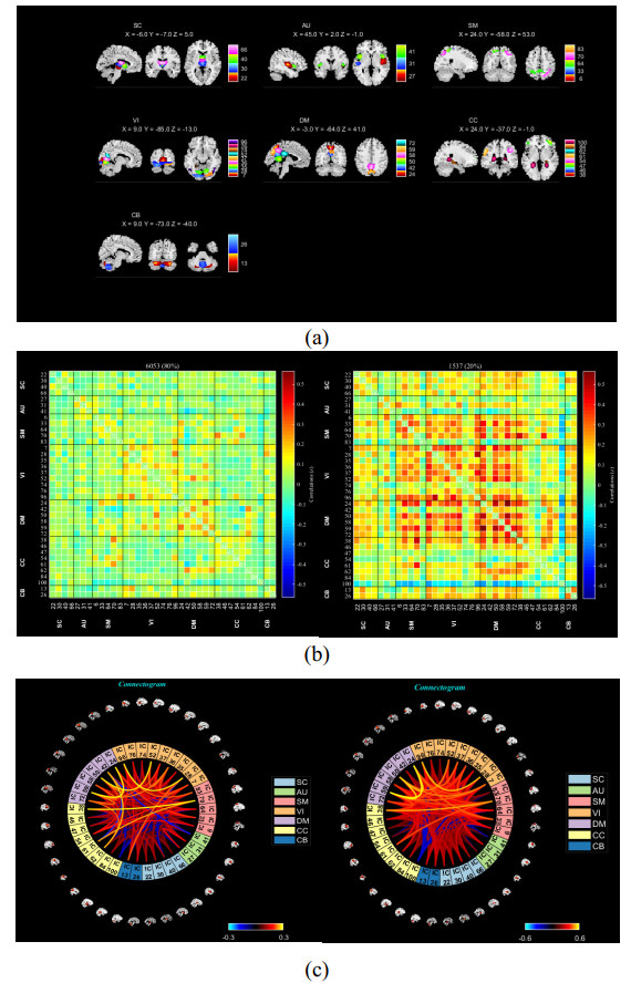
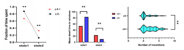
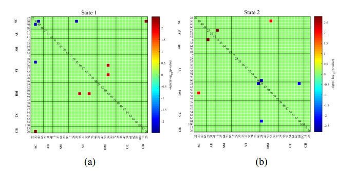
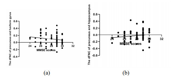
As is well known, the Apolipoprotein E (APOE) ε4 allele is the most pertinent genetic hazardous element for Alzheimer's disease (AD). Mild cognitive impairment (MCI) is considered a prodromal stage of AD. How the APOE ε4 allele modulates functional connectivity of brain network in MCI group is a question worth exploring. At present, some studies have evaluated the relationship between APOE ε4 allele and static functional network connectivity (sFNC) for MCI individuals, while the relationship of dynamic FNC (dFNC) with APOE ε4 allele still remained puzzled. Thus, we aim to detect aberrant dFNC for APOE ε4 carriers in the MCI group. On the basis of the resting-state functional magnetic resonance imaging (rs-fMRI) data, seven intrinsic brain functional networks were first recognized by the group independent component analysis. Then, the technique of sliding window was employed to determine the dFNC, and two dFNC states were detected by the k-means clustering algorithm. Finally, three temporal properties of fraction time, mean dwell time as well as transition numbers in the dFNC states were investigated. The results found that the dFNC and temporal properties in APOE ε4 carriers were abnormal compared with those in APOE ε4 noncarriers. In detail, in the MCI group, compared with APOE ε4 noncarriers, carriers had 9 pairs of abnormal dFNC and had significant differences in all the three temporal properties of the two dFNC states. In addition, two pairs of dFNC were found significantly correlated with clinical measure. This detected abnormal dynamics of temporal properties and dFNC in APOE ε4 carriers were similar with that reported for AD patients in previous studies. These results may suggest that in the MCI group, APOE carriers are more at risk for AD compared to noncarriers. Our findings may offer novel insights into the mechanisms of abnormal brain reconfiguration for individuals at genetic risk for AD, which could also be regarded as biomarkers for the early identification of AD.
Citation: Xiaoli Yang, Yan Liu. Abnormal dynamics of functional brain network in Apolipoprotein E ε4 carriers with mild cognitive impairment[J]. Electronic Research Archive, 2024, 32(1): 1-16. doi: 10.3934/era.2024001
As is well known, the Apolipoprotein E (APOE) ε4 allele is the most pertinent genetic hazardous element for Alzheimer's disease (AD). Mild cognitive impairment (MCI) is considered a prodromal stage of AD. How the APOE ε4 allele modulates functional connectivity of brain network in MCI group is a question worth exploring. At present, some studies have evaluated the relationship between APOE ε4 allele and static functional network connectivity (sFNC) for MCI individuals, while the relationship of dynamic FNC (dFNC) with APOE ε4 allele still remained puzzled. Thus, we aim to detect aberrant dFNC for APOE ε4 carriers in the MCI group. On the basis of the resting-state functional magnetic resonance imaging (rs-fMRI) data, seven intrinsic brain functional networks were first recognized by the group independent component analysis. Then, the technique of sliding window was employed to determine the dFNC, and two dFNC states were detected by the k-means clustering algorithm. Finally, three temporal properties of fraction time, mean dwell time as well as transition numbers in the dFNC states were investigated. The results found that the dFNC and temporal properties in APOE ε4 carriers were abnormal compared with those in APOE ε4 noncarriers. In detail, in the MCI group, compared with APOE ε4 noncarriers, carriers had 9 pairs of abnormal dFNC and had significant differences in all the three temporal properties of the two dFNC states. In addition, two pairs of dFNC were found significantly correlated with clinical measure. This detected abnormal dynamics of temporal properties and dFNC in APOE ε4 carriers were similar with that reported for AD patients in previous studies. These results may suggest that in the MCI group, APOE carriers are more at risk for AD compared to noncarriers. Our findings may offer novel insights into the mechanisms of abnormal brain reconfiguration for individuals at genetic risk for AD, which could also be regarded as biomarkers for the early identification of AD.

| [1] |
X. Liu, Q. Zeng, X. Luo, K. Li, H. Hong, S. Wang, et al., Effects of APOE ε2 on the fractional amplitude of low-frequency fluctuation in mild cognitive impairment: a study based on the resting-state functional MRI, Front. Aging Neurosci., 13 (2021), 1–11. https://doi.org/10.3389/fnagi.2021.591347 doi: 10.3389/fnagi.2021.591347

|
| [2] |
P. Liang, Z. Wang, Y. Yang, X. Jia, K. Li, Functional disconnection and compensation in mild cognitive impairment: evidence from DLPFC connectivity using resting-state fMRI, PLoS One, 6 (2011), e22153. https://doi.org/10.1371/journal.pone.0022153 doi: 10.1371/journal.pone.0022153
|
| [3] |
A. Chandra, P. E. Valkimadi, G. Pagano, O. Cousins, G. Dervenoulas, M. Politis, Applications of amyloid, tau, and neuroinflammation PET imaging to Alzheimer's disease and mild cognitive impairment, Hum. Brain Mapp., 40 (2019), 5424–5442. https://doi.org/10.1002/hbm.24782 doi: 10.1002/hbm.24782
|
| [4] |
C. Reitz, R. Mayeux, Alzheimer disease: epidemiology, diagnostic criteria, risk factors and biomarkers, Biochem. Pharmacol., 88 (2014), 640–651. https://doi.org/10.1016/j.bcp.2013.12.024 doi: 10.1016/j.bcp.2013.12.024
|
| [5] |
P. T. Nelson, I. Alafuzoff, E. H. Bigio, C. Bouras, H. Braak, N. J. Cairns, et al., Correlation of Alzheimer disease neuropathologic changes with cognitive status: a review of the literature, J. Neuropathol. Exp. Neurol., 71 (2012), 362–381. https://doi.org/10.1097/NEN.0b013e31825018f7 doi: 10.1097/NEN.0b013e31825018f7
|
| [6] |
J. Sheffler, J. Moxley, N. Sachs-Ericsson, Stress, race, and APOE: understanding the interplay of risk factors for changes in cognitive functioning, Aging Mental Health, 18 (2014), 784–791. https://doi.org/10.1080/13607863.2014.880403 doi: 10.1080/13607863.2014.880403
|
| [7] |
J. Raber, Y. Huang, J. W. Ashford, ApoE genotype accounts for the vast majority of AD risk and AD pathology, Neurobiol. Aging, 25 (2004), 641–650. https://doi.org/10.1016/j.neurobiolaging.2003.12.023 doi: 10.1016/j.neurobiolaging.2003.12.023
|
| [8] |
C. C. Liu, T. Kanekiyo, H. Xu, G. Bu, Apolipoprotein E and Alzheimer disease: risk, mechanisms and therapy, Nat. Rev. Neurol., 9 (2013), 184. https://doi.org/10.1038/nrneurol.2013.32 doi: 10.1038/nrneurol.2013.32
|
| [9] |
T. Li, B. Wang, Y. Gao, X. Wang, T. Yan, J. Xiang, et al., APOE ε4 and cognitive reserve effects on the functional network in the Alzheimer's disease spectrum, Brain Imaging Behav., 15 (2021), 758–771. https://doi.org/10.1007/s11682-020-00283-w doi: 10.1007/s11682-020-00283-w
|
| [10] |
B. C. Dickerson, R. A. Sperling, Large-scale functional brain network abnormalities in Alzheimer's disease: insights from functional neuroimaging, Behav. Neurol., 21 (2009), 63–75. https://doi.org/10.3233/BEN-2009-0227 doi: 10.3233/BEN-2009-0227
|
| [11] |
P. Wang, B. Zhou, H. Yao, Y. Zhan, Z. Zhang, Y. Cui, et al., Aberrant intra- and inter-network connectivity architectures in Alzheimer's disease and mild cognitive impairment, Sci. Rep., 5 (2015), 14824. https://doi.org/10.1038/srep14824 doi: 10.1038/srep14824
|
| [12] |
M. A. Binnewijzend, M. M. Schoonheim, E. Sanz-Arigita, A. M. Wink, W. M. van der Flier, N. Tolboom, et al., Resting-state fMRI changes in Alzheimer's disease and mild cognitive impairment, Neurobiol. Aging, 33 (2012), 2018–2028. https://doi.org/10.1016/j.neurobiolaging.2011.07.003 doi: 10.1016/j.neurobiolaging.2011.07.003
|
| [13] |
M. Sendi, E. Zendehrouh, Z. Fu, J. Liu, Y. Du, E. Mormino, et al., Disrupted dynamic functional network connectivity among cognitive control networks in the progression of Alzheimer's disease, Brain Connect., 13 (2023), 334–343. https://doi.org/10.1089/brain.2020.0847 doi: 10.1089/brain.2020.0847
|
| [14] |
M. Sendi, E. Zendehrouh, R. L. Miller, Z. Fu, Y. Du, J. Liu, et al., Alzheimer's disease projection from normal to mild dementia reflected in functional network connectivity: a longitudinal study, Front. Neural Circuits, 14 (2020). https://doi.org/10.3389/fncir.2020.593263 doi: 10.3389/fncir.2020.593263
|
| [15] |
J. Huang, P. Beach, A. Bozoki, D. C. Zhu, Alzheimer's disease progressively reduces visual functional network connectivity, J. Alzheimers Dis. Rep., 5 (2021), 549–562. https://doi.org/10.3233/ADR-210017 doi: 10.3233/ADR-210017
|
| [16] |
F. Tang, D. Zhu, W. Ma, Q. Yao, Q. Li, J. Shi, Differences changes in cerebellar functional connectivity between mild cognitive impairment and Alzheimer's disease: a seed-based approach, Front. Neurol., 12 (2021). https://doi.org/10.3389/fneur.2021.645171 doi: 10.3389/fneur.2021.645171
|
| [17] |
Q. Wang, C. He, Z. Wang, Z. Zhang, C. Xie, Dynamic connectivity alteration facilitates cognitive decline in Alzheimer's disease spectrum, Brain Connect., 11 (2021), 213–224. https://doi.org/10.1089/brain.2020.0823 doi: 10.1089/brain.2020.0823
|
| [18] |
G. Sanabria-Diaz, L. Melie-Garcia, B. Draganski, J. F. Demonet, F. Kherif, Apolipoprotein E4 effects on topological brain network organization in mild cognitive impairment, Sci. Rep., 11 (2021), 845. https://doi.org/10.1038/s41598-020-80909-7 doi: 10.1038/s41598-020-80909-7
|
| [19] |
H. Song, H. Long, X. Zuo, C. Yu, B. Liu, Z. Wang, et al., APOE effects on default mode network in Chinese cognitive normal elderly: relationship with clinical cognitive performance, PLoS One, 10 (2015), e0133179. https://doi.org/10.1371/journal.pone.0133179 doi: 10.1371/journal.pone.0133179
|
| [20] |
Y. Zhu, L. Gong, C. He, Q. Wang, Q. Ren, C. Xie, Default mode network connectivity moderates the relationship between the APOE genotype and cognition and individualizes identification across the Alzheimer's disease spectrum, J. Alzheimer's Dis., 70 (2019), 843–860. https://doi.org/10.3233/JAD-190254 doi: 10.3233/JAD-190254
|
| [21] |
P. A. Chiesa, E. Cavedo, A. Vergallo, S. Lista, M. C. Potier, M. O. Habert, et al., Differential default mode network trajectories in asymptomatic individuals at risk for Alzheimer's disease, Alzheimer's Dementia, 15 (2019), 940–950. https://doi.org/10.1016/j.jalz.2019.03.006 doi: 10.1016/j.jalz.2019.03.006
|
| [22] |
H. Lu, S. L. Ma, S. W. Wong, C. W. Tam, S. T. Cheng, S. S. Chan, et al., Aberrant interhemispheric functional connectivity within default mode network and its relationships with neurocognitivefeatures in cognitively normal APOE ε4 elderly carriers, Int. Psychogeriatrics, 29 (2017), 805–814. https://doi.org/10.1017/S1041610216002477 doi: 10.1017/S1041610216002477
|
| [23] |
M. M. Machulda, D. T. Jones, P. Vemuri, E. McDade, R. Avula, S. Przybelski, et al., Effect of APOE ε4 status on intrinsic network connectivity in cognitively normal elderly subjects, Arch. Neurol., 68 (2011), 1131–1136. https://doi.org/10.1001/archneurol.2011.108 doi: 10.1001/archneurol.2011.108
|
| [24] |
M. S. E. Sendi, E. Zendehrouh, C. A. Ellis, Z. Fu, J. Chen, R. L. Miller, et al., The link between static and dynamic brain functional network connectivity and genetic risk of Alzheimer's disease, Neuroimage: Clin., 37 (2023), 103363. https://doi.org/10.1016/j.nicl.2023.103363 doi: 10.1016/j.nicl.2023.103363
|
| [25] |
S. G. Mueller, M. W. Weiner, L. J. Thal, R. C. Petersen, C. R. Jack, W. Jagust, et al., Ways toward an early diagnosis in Alzheimer's disease: the Alzheimer's Disease Neuroimaging Initiative (ADNI), Alzheimer's Dementia, 1 (2005), 55–66. https://doi.org/10.1016/j.jalz.2005.06.003 doi: 10.1016/j.jalz.2005.06.003
|
| [26] |
C. G. Yan, Y. F. Zang, DPARSF: a MATLAB toolbox for "pipeline" data analysis of resting-state fMRI, Front. Syst. Neurosci., 4 (2010). https://doi.org/10.3389/fnsys.2010.00013 doi: 10.3389/fnsys.2010.00013
|
| [27] |
H. Chen, Z. Zou, X. Zhang, J. Shi, N. Huang, Y. Lin, Dynamic changes in functional network connectivity involving amyotrophic lateral sclerosis and its correlation with disease severity, J. Magn. Reson. Imaging, 54 (2021), 239–248. https://doi.org/10.1002/jmri.27521 doi: 10.1002/jmri.27521
|
| [28] |
Y. Gu, Y. Lin, L. Huang, J. Ma, J. Zhang, Y. Xiao, et al., Abnormal dynamic functional connectivity in Alzheimer's disease, CNS Neurosci. Ther., 26 (2020), 962–971. https://doi.org/10.1111/cns.13387 doi: 10.1111/cns.13387
|
| [29] |
J. Kim, M. Criaud, S. S. Cho, M. Díez-Cirarda, A. Mihaescu, S. Coakeley, et al., Abnormal intrinsic brain functional network dynamics in Parkinson's disease, Brain, 140 (2017), 2955–2967. https://doi.org/10.1093/brain/awx233 doi: 10.1093/brain/awx233
|
| [30] |
E. A. Allen, E. Damaraju, S. M. Plis, E. B. Erhardt, T. Eichele, V. D. Calhoun, Tracking whole-brain connectivity dynamics in the resting state, Cereb. Cortex, 24 (2014), 663–676. https://doi.org/10.1093/cercor/bhs352 doi: 10.1093/cercor/bhs352
|
| [31] |
G. Li, L. Zhou, Z. Chen, N. Luo, M. Niu, Y. Li, et al., Dynamic functional connectivity impairments in idiopathic rapid eye movement sleep behavior disorder, Parkinsonism Relat. Disord., 79 (2020), 11–17. https://doi.org/10.1016/j.parkreldis.2020.08.003 doi: 10.1016/j.parkreldis.2020.08.003
|
| [32] | S. Roweis, EM algorithms for PCA and SPCA, in Advances in Neural Information Processing Systems, 10 (1997), 626–632. Available from: https://proceedings.neurips.cc/paper_files/paper/1997/file/d9731321ef4e063ebbee79298fa36f56-Paper.pdf. |
| [33] |
A. J. Bell, T. J. Sejnowski, An information-maximization approach to blind separation and blind deconvolution, Neural Comput., 7 (1995), 1129–1159. https://doi.org/10.1162/neco.1995.7.6.1129 doi: 10.1162/neco.1995.7.6.1129
|
| [34] |
T. Yin, Z. He, P. Ma, R. Sun, K. Xie, T. Liu, et al., Aberrant functional brain network dynamics in patients with functional constipation, Hum. Brain Mapp., 42 (2021), 5985–5999. https://doi.org/10.1002/hbm.25663 doi: 10.1002/hbm.25663
|
| [35] |
Z. Yao, J. Shi, Z. Zhang, W Zheng, T. Hu, Y. Li, et al., Altered dynamic functional connectivity in weakly-connected state in major depressive disorder, Clin. Neurophysiol., 130 (2019), 2096–2104. https://doi.org/10.1016/j.clinph.2019.08.009 doi: 10.1016/j.clinph.2019.08.009
|
| [36] |
E. Agoalikum, B. Klugah-Brown, H. Yang, P. Wang, S. Varshney, B. Niu, et al., Differences in disrupted dynamic functional network connectivity among children, adolescents, and adults with attention deficit/hyperactivity disorder: a resting-state fMRI study, Front. Hum. Neurosci., 15 (2021). https://doi.org/10.3389/fnhum.2021.697696 doi: 10.3389/fnhum.2021.697696
|
| [37] |
X. Ma, X. Wu, Y. Shi, Changes of dynamic functional connectivity associated with maturity in late preterm infants, Front. Pediatr., 8 (2020). https://doi.org/10.3389/fped.2020.00412 doi: 10.3389/fped.2020.00412
|
| [38] |
J. Friedman, T. Hastie, R. Tibshirani, Sparse inverse covariance estimation with the graphical lasso, Biostatistics, 9 (2008), 432–441. https://doi.org/10.1093/biostatistics/kxm045 doi: 10.1093/biostatistics/kxm045
|
| [39] |
Q. Chen, J. Lu, X. Zhang, Y. Sun, W. Chen, X. Li, et al., Alterations in dynamic functional connectivity in individuals with subjective cognitive decline, Front. Aging Neurosci., 13 (2021). https://doi.org/10.3389/fnagi.2021.646017 doi: 10.3389/fnagi.2021.646017
|
| [40] |
R. P. Viviano, N. Raz, P. Yuan, J. S. Damoiseaux, Associations between dynamic functional connectivity and age, metabolic risk, and cognitive performance, Neurobiol. Aging, 59 (2017), 135–143. https://doi.org/10.1016/j.neurobiolaging.2017.08.003 doi: 10.1016/j.neurobiolaging.2017.08.003
|
| [41] |
L. Tian, Q. Li, C. Wang, J. Yu, Changes in dynamic functional connections with aging, Neuroimage, 172 (2018), 31–39. https://doi.org/10.1016/j.neuroimage.2018.01.040 doi: 10.1016/j.neuroimage.2018.01.040
|
| [42] |
K. Mevel, G. Chételat, F. Eustache, B. Desgranges, The default mode network in healthy aging and Alzheimer's disease, Int. J. Alzheimer's Dis., 2011 (2011), 535816. https://doi.org/10.4061/2011/535816 doi: 10.4061/2011/535816
|
| [43] |
Y. Zhan, J. Ma, A. F. Alexander-Bloch, K. Xu, Y. Cui, Q. Feng, et al., Longitudinal study of impaired intra- and inter-network brain connectivity in subjects at high risk for Alzheimer's disease, J. Alzheimer's Dis., 52 (2016), 913–927. https://doi.org/10.3233/JAD-160008 doi: 10.3233/JAD-160008
|
| [44] |
Y. I. Sheline, J. C. Morris, A. Z. Snyder, J. L. Price, Z. Yan, G. D'Angelo, et al., APOE4 allele disrupts resting state fMRI connectivity in the absence of amyloid plaques or decreased CSF Aβ42, J. Neurosci., 30 (2010), 17035–17040. https://doi.org/10.1523/JNEUROSCI.3987-10.2010 doi: 10.1523/JNEUROSCI.3987-10.2010
|
| [45] |
Z. Yao, B. Hu, J. Zheng, W. Zheng, X. Chen, X. Gao, et al., A FDG-PET study of metabolic networks in apolipoprotein E ε4 allele carriers, PLoS One, 10 (2015), e0132300. https://doi.org/10.1371/journal.pone.0132300 doi: 10.1371/journal.pone.0132300
|
| [46] |
C. Y. Lin, C. H. Chen, S. E. Tom, S. H. Kuo, Cerebellar volume is associated withcognitive decline in mild cognitive impairment: results from ADNI, Cerebellum, 19 (2020), 217–225. https://doi.org/10.1007/s12311-019-01099-1 doi: 10.1007/s12311-019-01099-1
|
| [47] |
M. Zhang, Z. Guan, Y. Zhang, W. Sun, W. Li, J. Hu, et al., Disrupted coupling between salience network segregation and glucose metabolism is associated with cognitive decline in Alzheimer's disease–a simultaneous resting-state FDG-PET/fMRI study, Neuroimage: Clin., 34 (2022), 102977. https://doi.org/10.1016/j.nicl.2022.102977 doi: 10.1016/j.nicl.2022.102977
|
| [48] |
G. Aghakhanyan, A. Vergallo, M. Gennaro, S. Mazzarri, F. Guidoccio, C. Radicchi, et al., The Precuneus–a witness for excessive Aβ gathering in Alzheimer's disease pathology, Neurodegener. Dis., 18 (2019), 302–309. https://doi.org/10.1159/000492945 doi: 10.1159/000492945
|
| [49] |
X. Tang, D. Holland, A. M. Dale, L. Younes, M. I. Miller, Shape abnormalities of subcortical and ventricular structures in mild cognitive impairment and Alzheimer's disease: detecting, quantifying, and predicting, Hum. Brain Mapp., 35 (2014), 3701–3725. https://doi.org/10.1002/hbm.22431 doi: 10.1002/hbm.22431
|
| [50] |
E. Lella, N. Amoroso, D. Diacono, A. Lombardi, T. Maggipinto, A. Monaco, et al., Communicability characterization of structural DWI subcortical networks in Alzheimer's disease, Entropy, 21 (2019), 475. https://doi.org/10.3390/e21050475 doi: 10.3390/e21050475
|
| [51] |
P. Mattila, T. Togo, D. W. Dickson, The subthalamic nucleus has neurofibrillary tangles in argyrophilic grain disease and advanced Alzheimer's disease, Neurosci. Lett., 320 (2002), 81–85. https://doi.org/10.1016/s0304-3940(02)00006-x doi: 10.1016/s0304-3940(02)00006-x
|
Figures(4) / Tables(3)
Xiaoli Yang, Yan Liu. Abnormal dynamics of functional brain network in Apolipoprotein E ε4 carriers with mild cognitive impairment[J]. Electronic Research Archive, 2024, 32(1): 1-16. doi: 10.3934/era.2024001


 DownLoad: