Feature fusion based artificial neural network model for disease detection of bean leaves

Eray Önler; Eray Önler

doi:10.3934/era.2023122

Electronic Research Archive

2023, Volume 31, Issue 5: 2409-2427. doi: 10.3934/era.2023122

Previous Article Next Article

Research article

Feature fusion based artificial neural network model for disease detection of bean leaves

Eray Önler ^,

Tekirdag Namik Kemal University, Faculty of Agriculture, Biosystem Engineering Department, Suleymanpasa, Tekirdag, Turkey

Received: 19 December 2022 Revised: 16 February 2023 Accepted: 23 February 2023 Published: 28 February 2023

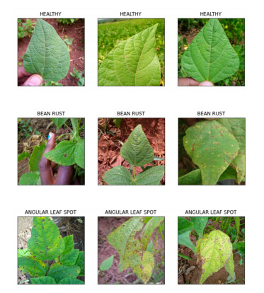
Plant diseases reduce yield and quality in agricultural production by 20–40%. Leaf diseases cause 42% of agricultural production losses. Image processing techniques based on artificial neural networks are used for the non-destructive detection of leaf diseases on the plant. Since leaf diseases have a complex structure, it is necessary to increase the accuracy and generalizability of the developed machine learning models. In this study, an artificial neural network model for bean leaf disease detection was developed by fusing descriptive vectors obtained from bean leaves with HOG (Histogram Oriented Gradient) feature extraction and transfer learning feature extraction methods. The model using feature fusion has higher accuracy than only HOG feature extraction and only transfer learning feature extraction models. Also, the feature fusion model converged to the solution faster. Feature fusion model had 98.33, 98.40 and 99.24% accuracy in training, validation, and test datasets, respectively. The study shows that the proposed method can effectively capture interclass distinguishing features faster and more accurately.
- leaf disease,
- artificial neural network,
- feature fusion,
- deep neural networks,
- computer vision
Citation: Eray Önler. Feature fusion based artificial neural network model for disease detection of bean leaves[J]. Electronic Research Archive, 2023, 31(5): 2409-2427. doi: 10.3934/era.2023122

Related Papers:

Abstract

Plant diseases reduce yield and quality in agricultural production by 20–40%. Leaf diseases cause 42% of agricultural production losses. Image processing techniques based on artificial neural networks are used for the non-destructive detection of leaf diseases on the plant. Since leaf diseases have a complex structure, it is necessary to increase the accuracy and generalizability of the developed machine learning models. In this study, an artificial neural network model for bean leaf disease detection was developed by fusing descriptive vectors obtained from bean leaves with HOG (Histogram Oriented Gradient) feature extraction and transfer learning feature extraction methods. The model using feature fusion has higher accuracy than only HOG feature extraction and only transfer learning feature extraction models. Also, the feature fusion model converged to the solution faster. Feature fusion model had 98.33, 98.40 and 99.24% accuracy in training, validation, and test datasets, respectively. The study shows that the proposed method can effectively capture interclass distinguishing features faster and more accurately.

References

[1]	G. S. Malhi, M. Kaur, P. Kaushik, Impact of climate change on agriculture and its mitigation strategies: A review, Sustainability, 13 (2021), 1318. https://doi.org/10.3390/su13031318 doi: 10.3390/su13031318
[2]	K. Yin, J. L. Qiu, Genome editing for plant disease resistance: applications and perspectives, Phil. Trans. R. Soc. B, 374 (2019), 20180322. https://doi.org/10.1098/rstb.2018.0322 doi: 10.1098/rstb.2018.0322
[3]	Z. Hu, What socio-economic and political factors lead to global pesticide dependence? A critical review from a social science perspective, Int. J. Environ. Res. Public Health, 17 (2020), 8119. https://doi.org/10.3390/ijerph17218119 doi: 10.3390/ijerph17218119
[4]	S. Roy, J. Halder, N. Singh, A. B. Rai, R. N. Prasad, B. Singh, Do vegetable growers really follow the scientific plant protection measures? An empirical study from eastern Uttar Pradesh and Bihar, Ind. J. Agric. Sci., 87 (2017), 1668–1672.
[5]	M. Ş. Şengül Demirak, E. Canpolat, Plant-based bioinsecticides for mosquito control: impact on insecticide resistance and disease transmission, Insects, 13 (2022), 162. https://doi.org/10.3390/insects13020162 doi: 10.3390/insects13020162
[6]	W. Cramer, J. Guiot, M. Fader, J. Garrabou, J. P. Gattuso, A. Iglesias, et al., Climate change and interconnected risks to sustainable development in the Mediterranean, Nat. Clim. Change, 8 (2018), 972–980. https://doi.org/10.1038/s41558-018-0299-2 doi: 10.1038/s41558-018-0299-2
[7]	H. N. Fones, D. P. Bebber, T. M. Chaloner, W. T. Kay, G. Steinberg, S. J. Gurr, Threats to global food security from emerging fungal and oomycete crop pathogens, Nat. Food, 1 (2020), 332–342. https://doi.org/10.1038/s43016-020-0075-0 doi: 10.1038/s43016-020-0075-0
[8]	M. Tudi, H. D. Ruan, L. Wang, J. Lyu, R. Sadler, D. Connell, et al., Agriculture development, pesticide application and its impact on the environment, Int. J. Environ. Res. Public Health, 18 (2021), 1112. https://doi.org/10.3390/ijerph18031112 doi: 10.3390/ijerph18031112
[9]	A. S. Tulshan, N. Raul, Plant leaf disease detection using machine learning, in 2019 10th International Conference on Computing, Communicatıon and Networkıng Technologıes (ICCCNT), 2019. https://doi.org/10.1109/ICCCNT45670.2019.8944556
[10]	A. Kumar, J. P. Singh, A. K. Singh, Randomized convolutional neural network architecture for eyewitness tweet identification during disaster, J. Grid Comput., 20 (2022). https://doi.org/10.1007/s10723-022-09609-y doi: 10.1007/s10723-022-09609-y
[11]	L. Xu, J. Xie, F. Cai, J. Wu, Spectral classification based on deep learning algorithms, Electronics, 10 (2021), 1892. https://doi.org/10.3390/electronics10161892 doi: 10.3390/electronics10161892
[12]	Ü. Atila, M. Uçar, K. Akyol, E. Uçar, Plant leaf disease classification using Efficient Net deep learning model, Ecol. Inf., 61 (2021), 101182. https://doi.org/10.1016/j.ecoinf.2020.101182 doi: 10.1016/j.ecoinf.2020.101182
[13]	S. Zhang, S. Zhang, C. Zhang, X. Wang, Y. Shi, Cucumber leaf disease identification with global pooling dilated convolutional neural network, Comput. Electron. Agric., 162 (2019), 422–430. https://doi.org/10.1016/j.compag.2019.03.012 doi: 10.1016/j.compag.2019.03.012
[14]	D. Jakubovitz, R. Giryes, M. R. Rodrigues, Generalization error in deep learning, in Compressed Sensing and Its Applications: Third International MATHEON Conference 2017, Birkhäuser, Cham, (2019), 153–193. https://doi.org/10.48550/arXiv.1808.01174
[15]	A. Al-Saffar, A. Bialkowski, M. Baktashmotlagh, A. Trakic, L. Guo, A. Abbosh, Closing the gap of simulation to reality in electromagnetic imaging of brain strokes via deep neural networks, IEEE Trans. Comput. Imaging, 7 (2020), 13–21. https://doi.org/10.1109/tci.2020.3041092 doi: 10.1109/tci.2020.3041092
[16]	G. Algan, I. Ulusoy, Image classification with deep learning in the presence of noisy labels: A survey, Knowl.-Based Syst., 215 (2021), 106771. https://doi.org/10.1016/j.knosys.2021.106771 doi: 10.1016/j.knosys.2021.106771
[17]	C. Wu, S. Guo, Y. Hong, B. Xiao, Y. Wu, Q. Zhang, Discrimination and conversion prediction of mild cognitive impairment using convolutional neural networks, Quant. Imaging Med. Surg., 8 (2018), 992. https://doi.org/10.21037/qims.2018.10.17 doi: 10.21037/qims.2018.10.17
[18]	K. Aderghal, A. Khvostikov, A. Krylov, J. Benois-Pineau, K. Afdel, G. Catheline, Classification of Alzheimer disease on imaging modalities with deep CNNs using cross-modal transfer learning, in 2018 IEEE 31st International Symposium on Computer-Based Medical Systems (CBMS), IEEE, (2018), 345–350. https://doi.org/10.1109/cbms.2018.00067
[19]	D. Chen, Y. Lu, Z. Li, S. Young, Performance evaluation of deep transfer learning on multi-class identification of common weed species in cotton production systems, Comput. Electron. Agric., 198 (2022), 107091. https://doi.org/10.1016/j.compag.2022.107091 doi: 10.1016/j.compag.2022.107091
[20]	M. Ahsan, M. A. Based, J. Haider, M. Kowalski, COVID-19 detection from chest X-ray images using feature fusion and deep learning, Sensors, 21 (2021), 1480. https://doi.org/10.3390/s21041480 doi: 10.3390/s21041480
[21]	L. Wei, K. Wang, Q. Lu, Y. Liang, H. Li, Z. Wang, et al., Crops fine classification in airborne hyperspectral imagery based on multi-feature fusion and deep learning, Remote Sens., 13 (2021), 2917. https://doi.org/10.3390/rs13152917 doi: 10.3390/rs13152917
[22]	C. Shang, F. Wu, M. Wang, Q. Gao, Cattle behavior recognition based on feature fusion under a dual attention mechanism, J. Visual Commun. Image Represent., 85 (2022), 103524. https://doi.org/10.1016/j.jvcir.2022.103524 doi: 10.1016/j.jvcir.2022.103524
[23]	H. C. Chen, A. M. Widodo, A. Wisnujati, M. Rahaman, J. C. W. Lin, L. Chen, et al., AlexNet convolutional neural network for disease detection and classification of tomato leaf, Electronics, 11 (2022), 951. https://doi.org/10.3390/electronics11060951 doi: 10.3390/electronics11060951
[24]	X. Fan, P. Luo, Y. Mu, R. Zhou, T. Tjahjadi, Y. Ren, Leaf image based plant disease identification using transfer learning and feature fusion, Comput. Electron. Agric., 196 (2022), 106892. https://doi.org/10.1016/j.compag.2022.106892 doi: 10.1016/j.compag.2022.106892
[25]	E. Elfatimi, R. Eryigit, L. Elfatimi, Beans leaf diseases classification using mobilenet models, IEEE Access, 10 (2022), 9471–9482. https://doi.org/10.1109/ACCESS.2022.3142817 doi: 10.1109/ACCESS.2022.3142817
[26]	S. S. Harakannanavar, J. M. Rudagi, V. I. Puranikmath, A. Siddiqua, R. Pramodhini, Plant leaf disease detection using computer vision and machine learning algorithms, Global Transitions Proc., 3 (2022), 305–310. https://doi.org/10.1016/j.gltp.2022.03.016 doi: 10.1016/j.gltp.2022.03.016
[27]	J. Annrose, N. Rufus, C. R. Rex, D. G. Immanuel, A cloud-based platform for soybean plant disease classification using archimedes optimization based hybrid deep learning model, Wireless Pers. Commun., 122 (2022), 2995–3017. https://doi.org/10.1007/s11277-021-09038-2 doi: 10.1007/s11277-021-09038-2
[28]	A. K. Singh, S. V. N. Sreenivasu, U. S. B. K. Mahalaxmi, H. Sharma, D. D. Patil, E. Asenso, Hybrid feature-based disease detection in plant leaf using convolutional neural network, Bayesian optimized SVM and random forest classifier, J. Food Qual., 2022 (2022). https://doi.org/10.1155/2022/2845320 doi: 10.1155/2022/2845320
[29]	Makerere AI Lab, Bean disease dataset, 2020. Available from: https://github.com/AI-Lab-Makerere/ibean.
[30]	A. Mikołajczyk, M. Grochowski, Data augmentation for improving deep learning in image classification problem, in 2018 International interdisciplinary PhD workshop (IIPhDW), IEEE, (2018), 117–122. https://doi.org/10.1109/iiphdw.2018.8388338
[31]	N. Dalal, B. Triggs, Histograms of oriented gradients for human detection, in 2005 IEEE Computer Society Conference on Computer Vision and Pattern Recognition (CVPR'05), 1 (2022), 886–893. https://doi.org/10.1109/cvpr.2005.177
[32]	S. van der Walt, J. L. Schönberger, J. Nunez-Iglesias, F. Boulogne, J. D. Warner, N. Yager, et al., scikit-image: Image processing in Python, PeerJ, 2014. https://doi.org/10.7287/peerj.preprints.336v2 doi: 10.7287/peerj.preprints.336v2
[33]	W. Samek, G. Montavon, S. Lapuschkin, C. J. Anders, K. R. Müller, Explaining deep neural networks and beyond: A review of methods and applications, Proc. IEEE, 109 (2021), 247–278. https://doi.org/10.1109/jproc.2021.3060483 doi: 10.1109/jproc.2021.3060483
[34]	Tensorflow Keras: Layers, Retrieved October 6, 2022. Available from: https://www.tensorflow.org/api_docs/python/tf/keras/layers.
[35]	D. P. Kingma, J. A. Ba, J. Adam, A method for stochastic optimization, preprint, arXiv: 1412.6980. https://doi.org/10.48550/arXiv.1412.6980
[36]	M. Sandler, A. Howard, M. Zhu, A. Zhmoginov, L. C. Chen, MobileNetV2: Inverted residuals and linear bottlenecks, in 2018 IEEE/CVF Conference on Computer Vision and Pattern Recognition, (2018), 4510–4520. https://doi.org/10.1109/cvpr.2018.00474
[37]	M. T. Riberio, S. Singh, C. Guestrin, "Why sould i trust you?" Explaining the predictions of any classifier, in Proceedings of the 22nd ACM SIGKDD international conference on knowledge discovery and data mining, (2016), 1135–1144. https://doi.org/10.1145/2939672.2939778
[38]	P. Bedi, P. Gole, PlantGhostNet: An efficient novel convolutional neural network model to identify plant diseases automatically, in 2021 9th International Conference on Reliability, Infocom Technologies and Optimization (Trends and Future Directions)(ICRITO), IEEE, (2021), 1–6. https://doi.org/10.1109/ICRITO51393.2021.9596543
[39]	A. Dosovitskiy, L. Beyer, A. Kolesnikov, D. Weissenborn, Z. Xiaohua, T. Unterthiner, et al., An image is wort 16x16 words: Transformers for image recognition at scale, preprint, arXiv: 2010.11929. https://doi.org/10.48550/arXiv.2010.11929
[40]	Y. Borhani, J. Khoramdel, E. Najafi, A deep learning based approach for automated plant disease classification using vision transformer, Sci. Rep., 12 (2022), 1–10. https://doi.org/10.1038/s41598-022-15163-0 doi: 10.1038/s41598-022-15163-0
[41]	Y. Lu, S. Young, A survey of public datasets for computer vision tasks in precision agriculture, Comput. Electron. Agric., 178, (2020), 105760. https://doi.org/10.1016/j.compag.2020.105760 doi: 10.1016/j.compag.2020.105760
[42]	X. Zhai, A. Kolesnikov, N. Houlsby, L. Beyer, Scaling vision transformers, in Proceedings of the IEE/CVF Conference on Computer Vision and Pattern Recognition, (2022), 12104–12113.
[43]	J. M. P. Czarnecki, S. Samiappan, M. Zhou, C. D. McCraine, L. L. Wasson, Real-time automated classification of sky conditions using deep learning and edge computing, Remote Sens., 13 (2021), 3859. https://doi.org/10.3390/rs13193859 doi: 10.3390/rs13193859
[44]	S. Yu, L. Xie, Q. Huang, Inception convolutional vision transformers for plant disease identification, Internet Things, 21 (2023), 100650. https://doi.org/10.1016/j.iot.2022.100650 doi: 10.1016/j.iot.2022.100650
[45]	H. Xu, X. Su, D. Wang, CNN-based local vision transformer for covid-19 diagnosis, preprint, arXiv: 2207.02027. https://doi.org/10.48550/arXiv.2207.02027

Reader Comments

Your name:*

Email:*
© 2023 the Author(s), licensee AIMS Press. This is an open access article distributed under the terms of the Creative Commons Attribution License (http://creativecommons.org/licenses/by/4.0)