Algorithms for solving a class of real quasi-symmetric Toeplitz linear systems and its applications

Xing Zhang; Xiaoyu Jiang; Zhaolin Jiang; Heejung Byun; Xing Zhang; Xiaoyu Jiang; Zhaolin Jiang; Heejung Byun

doi:10.3934/era.2023101

Electronic Research Archive

2023, Volume 31, Issue 4: 1966-1981. doi: 10.3934/era.2023101

Previous Article Next Article

Research article

Algorithms for solving a class of real quasi-symmetric Toeplitz linear systems and its applications

1.
School of Information Science and Technology, Linyi University, Linyi 276000, China
2.
College of Information Technology, The University of Suwon, Hwaseong-si 445-743, Republic of Korea
3.
School of Mathematics and Statistics, Linyi University, Linyi 276000, China

Received: 19 November 2022 Revised: 29 January 2023 Accepted: 29 January 2023 Published: 13 February 2023

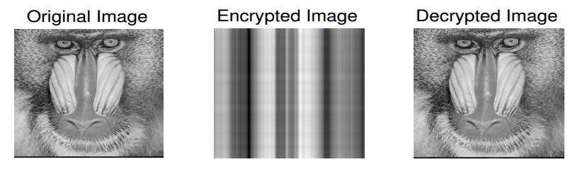
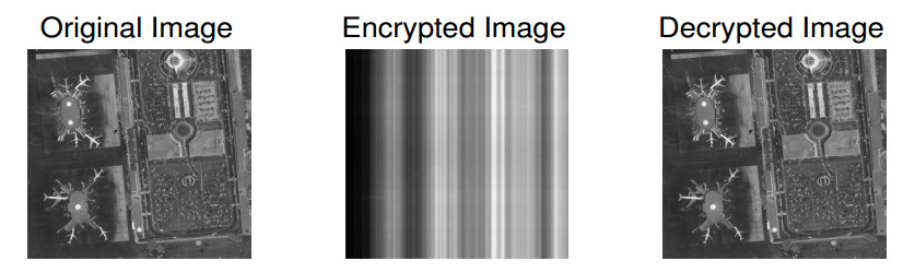
In this paper, fast numerical methods for solving the real quasi-symmetric Toeplitz linear system are studied in two stages. First, based on an order-reduction algorithm and the factorization of Toeplitz matrix inversion, a sequence of linear systems with a constant symmetric Toeplitz matrix are solved. Second, two new fast algorithms are employed to solve the real quasi-symmetric Toeplitz linear system. Furthermore, we show a fast algorithm for quasi-symmetric Toeplitz matrix-vector multiplication. In addition, the stability analysis of the splitting symmetric Toeplitz inversion is discussed. In mathematical or engineering problems, the proposed algorithms are extraordinarily effective for solving a sequence of linear systems with a constant symmetric Toeplitz matrix. Fast matrix-vector multiplication and a quasi-symmetric Toeplitz linear solver are proven to be suitable for image encryption and decryption.

Keywords:

Citation: Xing Zhang, Xiaoyu Jiang, Zhaolin Jiang, Heejung Byun. Algorithms for solving a class of real quasi-symmetric Toeplitz linear systems and its applications[J]. Electronic Research Archive, 2023, 31(4): 1966-1981. doi: 10.3934/era.2023101

Related Papers:

[1]	Kaiqing Huang, Yizhi Chen, Miaomiao Ren . Additively orthodox semirings with special transversals. AIMS Mathematics, 2022, 7(3): 4153-4167. doi: 10.3934/math.2022230
[2]	Tatjana Grbić, Slavica Medić, Nataša Duraković, Sandra Buhmiler, Slaviša Dumnić, Janja Jerebic . Liapounoff type inequality for pseudo-integral of interval-valued function. AIMS Mathematics, 2022, 7(4): 5444-5462. doi: 10.3934/math.2022302
[3]	Xuliang Xian, Yong Shao, Junling Wang . Some subvarieties of semiring variety COS $^{+}_{3}$ . AIMS Mathematics, 2022, 7(3): 4293-4303. doi: 10.3934/math.2022237
[4]	Johnny Henderson, Abdelghani Ouahab, Samia Youcefi . Existence results for ϕ-Laplacian impulsive differential equations with periodic conditions. AIMS Mathematics, 2019, 4(6): 1610-1633. doi: 10.3934/math.2019.6.1610
[5]	Liaqat Ali, Yaqoub Ahmed Khan, A. A. Mousa, S. Abdel-Khalek, Ghulam Farid . Some differential identities of MA-semirings with involution. AIMS Mathematics, 2021, 6(3): 2304-2314. doi: 10.3934/math.2021139
[6]	Fenhong Li, Liang Kong, Chao Li . Non-global nonlinear mixed skew Jordan Lie triple derivations on prime $\ast$ -rings. AIMS Mathematics, 2025, 10(4): 7795-7812. doi: 10.3934/math.2025357
[7]	Xia Li, Wen Guan, Da-Bin Wang . Least energy sign-changing solutions of Kirchhoff equation on bounded domains. AIMS Mathematics, 2022, 7(5): 8879-8890. doi: 10.3934/math.2022495
[8]	Liang Kong, Chao Li . Non-global nonlinear skew Lie triple derivations on factor von Neumann algebras. AIMS Mathematics, 2022, 7(8): 13963-13976. doi: 10.3934/math.2022771
[9]	Heng Yang, Jiang Zhou . Compactness of commutators of fractional integral operators on ball Banach function spaces. AIMS Mathematics, 2024, 9(2): 3126-3149. doi: 10.3934/math.2024152
[10]	Wenbo Huang, Jiankui Li, Shaoze Pan . Some zero product preserving additive mappings of operator algebras. AIMS Mathematics, 2024, 9(8): 22213-22224. doi: 10.3934/math.20241080

Abstract

1. Introduction

Discrete lifetime data—such as the number of appliance failures of a particular brand within a given time frame, the total number of machine operations prior to a failure, the number of bullets fired by a weapon before the first malfunction, and the anticipated lifespan of humans (in years)—are frequently handled in reliability lifetime studies. For more classic examples, see Szymkowiak and Iwinska ^[1]. Data scientists typically employ discrete models as analysis tools, such as the Poisson distribution, negative binomial distribution, and geometric distribution, in order to more correctly define, analyze, and model these data. But in many situations, these discrete distribution functions are not the best options. For instance, seasonal or periodic data cannot be handled by the Poisson distribution, while underdispersed data cannot be described by the negative binomial distribution. More suitable discrete lifetime distributions are required to explore many additional kinds of complex discrete lifespan data. Discretizing continuous random variables is a useful strategy that yields a discrete life model with characteristics that are comparable to the continuous model.

The essential concept of discretizing continuous random variables was first presented by Roy ^[2]. Specifically, let $Y$ be a continuous random variable with a survival function denoted by $S(y)$ . Define the random variable $Z = [Y]$ as the maximum integer less than or equal to $Y$ . The probability mass function (PMF) $P(Z = z)$ of $Z$ can be expressed as

$\begin{align*} P(Z = z) = S_Y(z)-S_Y(z+1). \end{align*}$

Many researchers have introduced various new models for discrete life distributions by the approach. For instance, the discrete normal distribution was first introduced by Roy ^[3]. Using the generic method of discretizing a continuous distribution, Krishna and Pundir ^[4] introduced the discrete Burr and Pareto distributions. In addition, Bracquemond and Gaudoin ^[5] provided an extensive overview of discrete distributions, such as the Weibull distribution, that are employed in reliability to describe discrete lifetimes of nonrepairable systems. It is well-known that the Weibull distribution has become the most commonly used distribution for analyzing continuous life data due to its ability to fit various types of data and relatively simple structure (Johnson et al. ^[6]). At least three cases exist for the corresponding discrete Weibull distribution: (a) the Type Ⅰ discrete Weibull distribution, which maintains the form of the continuous survival function (SF), as introduced by Nakagawa and Osaki ^[7]; (b) the Type Ⅱ discrete Weibull distribution, as suggested by Stein and Dattero ^[8]; and (c) the three-parameter discrete Weibull distribution, as introduced by Padgett and Spurrier ^[9]. The most popular of them is the Type Ⅰ discrete Weibull distribution, whose features have been extensively researched by numerous academics. Englehardt and Li ^[10] employed the discrete Weibull distribution to analyze pathogen counts in treated water over time. Barbiero ^[11,12] compared several parameter estimation methods of this distribution, and solved the minimum Chi-square and least squares estimation. Vila et al. ^[13] studied in detail the basic theoretical properties of the Type Ⅰ discrete Weibull and analyzed the censored data. Yoo ^[14] extended the application of the discrete Weibull regression model to accommodate missing data. In addition, El-Morshedy et al. ^[15] conducted a detailed study on a new bivariate exponential discrete Weibull distribution.

The primary goal in this study is to enhance the current techniques for estimating the complex discrete probability distribution model. The probability distribution's score function typically lacks an explicit analytical solution, hence the Newton approach is usually used to estimate the numerical solution for parameter estimation. Nevertheless, the algorithm's low convergence and strong dependence on the initial value make it challenging to achieve the best estimation outcomes. Recently, Liu et al. ^[16] employed the majorize minimize (MM) algorithm to enhance the resolution of the maximum likelihood estimation for the simplex distribution. Li and Tian ^[17] introduced a novel root-finding method known as the upper-crossing/solution (US) algorithm. In contrast to conventional iterative algorithms (like Newton's algorithm), the US algorithm can lessen the influence of initial values and achieve a strong, stable convergence to the objective equation's real root at each iteration. The benefits of this technique have been illustrated through the use of a few classic models, such as the Weibull distribution, gamma distribution, zeta distribution, and generalized Poisson distribution. Cai ^[18] has improved the maximum likelihood estimation of generalized gamma distribution parameters by combining the US algorithm with the second-derivative lower-bound function (SeLF) algorithm.

The essence of the US algorithm is to identify a $U$ -function $U(\theta|\theta^{(t)})$ , which simplifies the solution of the complicated nonlinear equation $h(\theta) = 0$ to the solution of the equation $U(\theta|\theta^{(t)}) = 0$ with an explicit solution. Li and Tian ^[17] presented a variety of approaches to discover the $U$ -function, among which the first-derivative lower bound (FLB) function method requires only by using the first derivative of the objective function $h(\theta)$ , thereby diminishing algorithmic complexity. In previous research on the US algorithm, it was generally used to solve the roots of univariate nonlinear equations or the maximum likelihood estimation problem of a multi-parameter probability distribution with an explicit partial score function. Specifically, for a probability distribution with two parameters $(\alpha, \beta)$ , while solving for maximum likelihood estimation, the estimator of the parameter $\alpha$ can be explicitly expressed by the other estimator of the parameter $\beta(\alpha)$ . However, there is no further discussion provided in Li and Tian ^[17] about whether this approach can be applicable in more complex multi-parameter distributions, where an estimator of one parameter cannot be clearly represented by the other, and it is an issue deserving of more investigation.

The rest of the paper will proceed as follows. Section 2 provides a detailed introduction to the US algorithm and FLB function method. The application of the suggested approach to the Type Ⅰ discrete Weibull distribution's maximum likelihood parameter estimation is covered in Section 3. Numerical simulation experiments will be conducted in Section 4 in order to evaluate the performance of the employed methods and compare them with alternative estimation approaches. Section 5 will demonstrate the applicability of the US algorithm through the analysis of two real data sets. Conclusions and discussions will be provided in Section 6.

2. The US algorithm

One of the most frequent issues in numerical computations is figuring out the zero point of a function or an equation's root. In classical statistics, the maximum likelihood estimate (MLE) of parameters and the calculation of maximum a posteriori probability in Bayesian statistics may typically be turned into the problem of solving the zero point of a nonlinear function $h (\theta)$ . In summary, since $h(\theta)$ is a nonlinear function of a single variable $\theta$ , we must identify the unique root $\theta^\star$ such that

$\begin{equation} h(\theta) = 0,\qquad \theta \in \Theta \subseteq \mathbb{R}. \end{equation}$

(2.1)

The US algorithm is the most recent method for discovering roots. It has a similar procedure to the commonly used EM (expectation maximum) and MM (maximize minimize) algorithms^[17]. There are two primary steps in this process: the upper-crossing step (U-step) and the solution step (S-step). The two primary advantages of this algorithm are as follows:

(a) It converges strongly and stably to the root $\theta^\star$ of the Eq (2.1) with each iteration, that is, for an iterative points set sequence $\left\{\theta^{(t)} \right\}^{\infty}_{t = 0}$ , there is

$\theta^{(0)} < \theta^{(1)} < \cdots < \theta^{(t)} < \cdots\leq \theta^\star \quad or \quad \theta^\star \leq \cdots < \theta^{(t)} < \cdots < \theta^{(1)} < \theta^{(0)}.$

(b) The Newton algorithm's sensitivity to the initial value is decreased.

Two new symbols, $\overset{sgn(\alpha)}{\leq}$ and $\overset{sgn(\alpha)}{\geq}$ , are introduced regarding the changing direction (CD) inequalities in order to simplify the explanation of the US algorithm. The specific definition is presented as follows: for two functions $f_1(x)$ and $f_2(x)$ on the same domain $\mathbb{Q}$ ,

$f_1(x)\overset{sgn(\alpha)}{\leq}f_2(x) \Leftrightarrow \left\{\begin{aligned} f_1(x)\leq f_2(x), \qquad \alpha > 0,\\ f_1(x) = f_2(x), \qquad \alpha = 0,\\ f_1(x)\geq f_2(x), \qquad \alpha < 0, \end{aligned}\right.$

and

$f_1(x)\overset{sgn(\alpha)}{\geq}f_2(x) \Leftrightarrow \left\{\begin{aligned} f_1(x)\geq f_2(x), \qquad \alpha > 0,\\ f_1(x) = f_2(x), \qquad \alpha = 0,\\ f_1(x)\leq f_2(x), \qquad \alpha < 0. \end{aligned}\right.$

2.1. Definition of the U-function

It is typically challenging to locate the root $\theta^\star$ of the nonlinear equation $h(\theta) = 0$ directly. The US algorithm aims to create an alternative function $U(\theta|\theta^{(T)})$ to replace $h (\theta)$ , transforming the challenge of solving complex nonlinear equations into solving the equation $U(\theta|\theta^{(T)})$ with explicit solutions. First, we assume that

$\begin{equation} \begin{aligned} h(\theta) < 0,\quad \forall \theta > \theta^\star \ and \ h(\theta) > 0,\quad \forall \theta < \theta^\star. \end{aligned} \end{equation}$

(2.2)

If $h(\theta) < 0$ when $\theta < \theta^\star$ , then both sides of the equation $h(\theta) = 0$ can be multiplied by -1, which can also obtain the same root $\theta^\star$ satisfying the assumption (2.2). Let $\theta^{(t)}$ represent the solution after the ( $t$ -1)-th iteration, and the function $U(\theta|\theta^{(t)})$ satisfying the following criteria is designated as the U-function of $h(\theta)$ at $\theta = \theta^{(t)}$ :

$\begin{equation} \begin{aligned} h(\theta)\quad\leq \quad&U(\theta|\theta^{(t)}),\qquad&\theta < \theta^{(t)},\\ h(\theta^{(t)})\quad = \quad&U(\theta^{(t)}|\theta^{(t)}),\qquad& \theta = \theta^{(t)},\\ h(\theta)\quad\geq \quad&U(\theta|\theta^{(t)}),\qquad&\theta > \theta^{(t)}. \end{aligned} \end{equation}$

(2.3)

According to the definition of the CD inequalities symbol, the above condition may be represented as

$\begin{equation} h(\theta)\overset{sgn(\theta-\theta^{(t)})}{\geq}U(\theta|\theta^{(t)}),\qquad \forall \theta,\theta^{(t)}\in \Theta. \end{equation}$

(2.4)

2.2. The U-equation

As described above, the US algorithm is an iterative approach for solving nonlinear equations, with each iteration including a U-step and an S-step. The purpose of the U-step is to find a U-function that satisfies the condition (2.4), whereas the S-step involves solving the simplified U-equation: $U(\theta|\theta^{(t)}) = 0$ to obtain its root $\theta^{(t+1)}$ ,

$\begin{equation} \theta^{(t+1)} = sol\left\{U(\theta|\theta^{(t)}) = 0,\quad\forall\theta,\theta^{(t)}\in\Theta \right\}. \end{equation}$

(2.5)

In typical scenarios, $\theta^{(t+1)}$ can be explicitly expressed, even as a linear equation. Through the iterative execution of these two steps, $\left\{\theta^{(t)} \right\}^{\infty}_{t = 0}$ can gradually converge to the real root $\theta^\star$ of the U-equation.

2.3. The first-derivative lower bound function method

There are numerous U-functions for a given objective function $h(\theta)$ ; as Eq (2.4) illustrates, distinct U-functions correlate to distinct US algorithms. We may express the U-function using the lower-order derivatives of the goal function $h(\theta)$ . This can be accomplished by a variety of techniques, such as the first-derivative lower bound (FLB), second-derivative lower-upper bound (SLUB) constants method, and third-derivative lower bound (TLB) constant method ^[17]. These three methodologies enhance efficient solutions when the objective function is complex and the solution is not closed, each with a distinct convergence speed. In terms of maximizing the objective function, the US algorithm based on the FLB approach shares qualities with the EM algorithm and the MM algorithm, both of which exhibit linear convergence. The FLB function technique, which is dependent on the target function's first-order derivative, is mostly used in this article to generate the required U-function. First for parameter space $\Theta$ , we suppose that there exists a certain first-derivative lower bound function $b(\theta)$ for the first derivative of $h(\theta)$ , i.e.,

$\begin{equation} \begin{aligned} h^\prime(\theta)\geq b(\theta),\quad \forall\theta \in\Theta. \end{aligned} \end{equation}$

(2.6)

The U-function of $h(\theta)$ at $\theta = \theta^{(t)}$ can be formally defined as follows

$\begin{equation} \begin{aligned} U(\theta|\theta^{(t)})\overset{\Delta}{ = }h(\theta^{(t)})+\int^\theta_{\theta^{(t)}}b(z)\rm d z,\quad\forall \theta,\theta^{(t)}\in\Theta. \end{aligned} \end{equation}$

(2.7)

In fact,

$\begin{equation} \begin{aligned} h(\theta)-U(\theta|\theta^{(t)})\quad& = \quad [h(\theta)-h(\theta^{(t)})]-\int^\theta_{\theta^{(t)}}b(z)\rm d z = \int^\theta_{\theta^{(t)}}\textit h^\prime(z)\rm d z-\int^\theta_{\theta^{(t)}}\textit b(z)\rm d z \\[0.5cm]& = \quad \int^\theta_{\theta^{(t)}}[h^\prime(z)-b(z)]\rm d z \quad\overset{sgn(\theta-\theta^{(t)})}{\geq} 0 , \quad \forall \theta,\theta^{(t)}\in\Theta. \end{aligned} \end{equation}$

Let $\theta^\star$ be the unique root of the equation $h(\theta) = 0$ , and then the corresponding US iteration is as follows:

$\begin{equation} \begin{aligned} \theta^{(t+1)} = \quad sol\left\{U(\theta|\theta^{(t)}) = h(\theta^{(t)})+\int_{\theta^{(t)}}^{\theta}b(z)\rm d z = 0,\forall \theta,\theta^{(t)} > 0\right\}\overset{\Delta}{ = }g(\theta^{(t)}), \end{aligned} \end{equation}$

(2.8)

where $g(\theta^{(t)}) = g(\theta^\star)+(\theta^{(t)}-\theta^\star)h^\prime(\theta^\star)+0.5(\theta^{(t)}-\theta^\star)^2h^{\prime\prime}(\hat{\theta})$ is the first-order Taylor expansion around $\theta^\star$ , and $\theta^\star$ is a point between $\theta^{(t)}$ and $\theta^\star$ .

Although Li and Tian ^[17] proposed the idea of the US algorithm, in practical applications, only the distribution of univariate and binary parameters were studied. In the case of binary parameter distribution, when discussing the solution of the scoring equation, only one parameter can be explicitly expressed with another parameter. However, when one parameter cannot be explicitly expressed by the other parameter for this more general and complex situation, whether the US algorithm can be effectively applied is not further discussed, which is the issue to be carried out in this article. For the parameters of interest, the new FLB functions are constructed in this article, then, starting with initial values, the iterative values are updated using the corresponding S-step until the convergence criteria are met.

3. The US algorithm for the MLE of the Type Ⅰ discrete Weibull distribution

The discrete Weibull distribution's score function has a complex double exponential form, which makes it impossible to depict its solution and, thus, prevents its two parameters from being mutually expressed. For investigating the US algorithm's applicability in complicated models, we combine the US algorithm with the FLB method in this section to optimize the maximum likelihood estimation.

3.1. The Type Ⅰ discrete Weibull distribution

Assuming a random variable following the Weibull distribution $W(\lambda, \beta)$ , where $\lambda > 0$ and $\beta > 0$ , the cumulative distribution function (CDF) of the Weibull distribution is defined as $H\left(t, \lambda, \beta\right) = 1-e^{-\lambda t^\beta}$ , where $t > 0$ . Define $\alpha = e^{-\lambda}$ , and then $0 < \alpha < 1$ . If the probability mass function (PMF) for a random variable $X$ can be represented as

$\begin{equation} P(X = x;\alpha,\beta) = \alpha^{([x]-1)^\beta}-\alpha^{[x]^\beta},(x\geq1), \end{equation}$

then we say that $X$ follows the Type Ⅰ discrete Weibull distribution, denoted as $X\sim DW(\mathit{\boldsymbol{\theta)}}$ . Here, $[x]$ represents the maximum integer less than or equal to $x$ . When $\beta$ = 1, the discrete Weibull distribution degenerates to the geometric distribution $Geo(q)$ with $q = 1-\alpha$ .

Naturally, the cumulative distribution function of $X$ takes the following form:

$\begin{equation} F(x;\alpha,\beta) = 1-\alpha^{[x]^\beta}. \end{equation}$

3.2. The US algorithm for the MLE of $\alpha$ and $\beta$

This section will go into detail on the application of the US algorithm for maximum likelihood estimation of the Type Ⅰ discrete Weibull distribution. Assume $X$ is a random variable with the Type Ⅰ discrete Weibull distribution $DW(\mathit{\boldsymbol{\theta}})$ , where the parameter vector $\mathit{\boldsymbol{\theta}} = (\alpha, \beta)^T$ is in the parameter space $\Theta \subset \mathbb{R}^2$ . Let $\textbf{x} = (x_1, ..., x_n)$ denote the observed values of the random sample $(X_1, ..., X_n)$ . Then, the log-likelihood function of the parameter vector $\mathit{\boldsymbol{\theta}}$ is given by

$\ell(\mathit{\boldsymbol{\theta}}|\textbf{x}) = \sum\limits_{i = 1}^{n}\log(\alpha^{(x_i-1)^\beta}-\alpha^{(x_i)^\beta}).$

First, the first-order partial derivative of $\ell(\mathit{\boldsymbol{\theta}}|\textbf{x})$ with respect to $\alpha$ can be calculated as

$\begin{equation} \frac{\partial\ell(\mathit{\boldsymbol{\theta}}|\textbf{x})}{\partial\alpha} = \sum\limits_{i = 1}^{n}\alpha^{-1}\left[\frac{\alpha^{(x_i-1)^\beta}(x_i-1)^\beta-\alpha^{x_i^\beta}x_i^\beta}{\alpha^{(x_i-1)^\beta}-\alpha^{x_i^\beta}}\right]\overset{\Delta}{ = }h_1(\alpha). \end{equation}$

(3.1)

Next, we construct the FLB function regarding the parameter $\alpha$ :

$\begin{equation} \begin{aligned} h_1^\prime(\alpha)& = \sum\limits_{i = 1}^{n}\frac{\left[[(x_i-1)^\beta-1](x_i-1)^\beta\alpha^{(x_i-1)^\beta-2}-(x_i^\beta-1)x_i^\beta\alpha^{x_i^\beta-2}\right](\alpha^{(x_i-1)^\beta}-\alpha^{x_i^\beta})}{(\alpha^{(x_i-1)^\beta}-\alpha^{x_i^\beta})^2} \\[0.5cm]&-\sum\limits_{i = 1}^{n}\frac{\left[\alpha^{(x_i-1)^\beta}(x_i-1)^\beta-\alpha^{x_i^\beta-1}x_i^\beta\right]((x_i-1)^\beta\alpha^{(x_i-1)^\beta-1}-x_i^\beta\alpha^{x_i^\beta-1})}{(\alpha^{(x_i-1)^\beta}-\alpha^{x_i^\beta})^2} \\[0.5cm]&\geq-\sum\limits_{i = 1}^{n}\frac{\left[\alpha^{2(x_i-1)^\beta-2}[(x_i-1)^\beta+(x_i-1)^{2\beta}]+\alpha^{x_i^\beta+(x_i-1)^\beta-2}[(x_i-1)^{2\beta}+x_i^{2\beta}]+\alpha^{2x_i^\beta-2}[x_i^{2\beta+x_i^\beta}]\right]}{(\alpha^{(x_i-1)^\beta}-\alpha^{x_i^\beta})} \\[0.5cm]&\geq-\sum\limits_{i = 1}^{n}\alpha^{2(x_i-1)^\beta-2}\frac{[2(x_i-1)^{2\beta}+2x_i^{2\beta}+(x_i-1)^\beta+x_i^\beta]}{(\alpha^{(x_i-1)^\beta}-\alpha^{x_i^\beta})^2} \\[0.5cm]&\geq-\sum\limits_{i = 1}^{n}\frac{4x_i^{2\beta}+2x_i^\beta}{(\alpha-\alpha^2)^2} = -\sum\limits_{i = 1}^{n}3[4x_i^{2\beta}+2x_i^\beta]\left[\frac{1}{\alpha^2}+\frac{1}{(1-\alpha)^2}\right]\overset{\Delta}{ = }b_1(\alpha). \end{aligned} \end{equation}$

(3.2)

Then, the US iteration of $\alpha$ can be obtained as follows:

$\begin{equation} \begin{aligned} \alpha^{(t+1)}& = sol\left[U_\alpha(\alpha,\beta|\alpha^{(t)},\beta^{(t)}) = h_1(\alpha^{(t)})+\int^\alpha_{\alpha^{(t)}}b_1(z)\rm d z = 0\right] \\[0.5cm]& = sol\left[C_1+3C_2\left[\frac{1}{\alpha}-\frac{1}{1-\alpha}\right]-3C_2\left[\frac{1}{\alpha^{(t)}}-\frac{1}{1-\alpha^{(t)}}\right] = 0]\right] \\[0.5cm]& = sol\left[(C_3-C_1)\alpha^2-(6C_2+C_3-C_1)\alpha+3C_2 = 0\right], \end{aligned} \end{equation}$

(3.3)

where $C_1 = h_1(\alpha^{(t)})$ , $C_2 = \sum_{i = 1}^{n}[4x_i^{2\beta^{(t)}}+2x_i^{\beta^{(t)}}]$ , and $C_3 = 3C_2\left[\frac{1}{\alpha^{(t)}}-\frac{1}{1-\alpha^{(t)}}\right]$ . Similarly, we can obtain the first-order partial derivative of $\ell(\mathit{\boldsymbol{\theta}}|\textbf{x})$ with respect to $\beta$ ,

$\begin{equation} \frac{\partial\ell(\mathit{\boldsymbol{\theta}}|\textbf{x})}{\partial\beta} = \sum\limits_{i = 1}^{n}\log\alpha\left[\frac{\alpha^{(x_i-1)^\beta}(x_i-1)^\beta \log(x_i-1)-\alpha^{x_i^\beta}x_i^\beta \log(x_i)}{\alpha^{(x_i-1)^\beta}-\alpha^{x_i^\beta}}\right]\overset{\Delta}{ = }h_2(\beta). \end{equation}$

(3.4)

In order to construct the FLB function and derive the US algorithm without explicit solutions for the two parameters, we need the following two lemmas.

Lemma 1. ^[18] Given that $\theta > 0$ , we have

$-e^\theta\geq-\frac{4e^{2max(\theta^{(t)}-1,0)}}{(2\theta^{(t)}-\theta)^2},\quad\forall0\leq\theta\leq2\theta^{(t)} \quad and\quad \theta^{(t)} > 0.$

Lemma 2. ^[18] For any $\theta\geq0$ , we have

$-e^{-\theta}\geq-\frac{2}{3}\theta^{-2}.$

We will then build the FLB function with respect to $\beta$ . First, we calculate $h_2(\beta)$ 's first derivative.

$\begin{equation} \begin{aligned} h_2^\prime(\beta)& = \sum\limits_{i = 1}^{n}\log(\alpha)\frac{\left[\log^2(x_i-1)(x_i-1)^{2\beta}\alpha^{2(x_i-1)^\beta}(1-\log\alpha)+\log^2(x_i)x_i^{2\beta}\alpha^{2(x_i-1)^\beta}(1-\log(\alpha))\right]}{(\alpha^{(x_i-1)^\beta}-\alpha^{x_i^\beta})^2} \\[0.5cm]&+\sum\limits_{i = 1}^{n}\log(\alpha)\frac{\left[2\log(\alpha)\log(x_i)\log(x_i-1)x_i^\beta(x_i-1)^\beta-\log^2(x_i-1)(x_i-1)^\beta-\log^2(x_i)x_i^\beta\right]\alpha^{2x_i^\beta}}{(\alpha^{(x_i-1)^\beta}-\alpha^{x_i^\beta})^2} \\[0.5cm]&\geq\sum\limits_{i = 1}^{n}\frac{\left[2\log^2(x_i)x_i^{2\beta}\alpha^{2(x_i-1)^\beta}[1-\log(\alpha)]-2\log^2(x_i-1)(x_i-1)^\beta\alpha^{2x_i^\beta}[1-\log(\alpha)]\right]}{(\alpha^{(x_i-1)^\beta}-\alpha^{x_i^\beta})} \\[0.5cm]&\geq\sum\limits_{i = 1}^{n}\frac{2\log(\alpha)(1-\log(\alpha))\log^2(x_i)x_i^{2\beta}\alpha^{2(x_i-1)^\beta}}{(\alpha^{(x_i-1)^\beta}-\alpha^{x_i^\beta})^2} \\[0.5cm]&\geq-\frac{2\log(\alpha)(1-\log(\alpha))}{[1-\alpha]^2}\left[-\sum\limits_{i = 1}^{n}\log^2(x_i)x_i^{2\beta}\right]. \end{aligned} \end{equation}$

It can be deduced from Lemma 1 and Lemma 2 that

$\begin{equation} \begin{aligned} &-\sum\limits_{i = 1}^{n}\log^2(x_i)x_i^{2\beta} = -\sum\limits_{i = 1}^{n}e^{2\beta\log(x_i)}\log^2(x_i) \\[0.5cm]\geq&-\sum\limits_{i = 1}^{n}\left[\frac{4e^{2max(2\beta^{(t)}\log(x_i)-1,0)}I(\log(x_i) > 0)}{\left[4\beta^{(t)}\log(x_i)-2\beta\right]^2}+\frac{2I(\log(x_i)\leq0)}{3[-2\beta\log(x_i)]^2}\right]\log^2(x_i) \\[0.5cm] = &-\sum\limits_{i = 1}^{n}\left[\frac{4e^{2max(2\beta^{(t)}\log(x_i)-1,0)}I(x_i > 1)}{(4\beta^{(t)}-2\beta)^2}+\frac{I(x_i = 1)}{6\beta^2}\right], \end{aligned} \end{equation}$

where $I(\cdot)$ is the indicator function. Then, the corresponding FLB function is obtained as follows:

$\begin{equation} \begin{aligned} \frac{2\log(\alpha)(1-\log(\alpha))}{[1-\alpha]^2}\sum\limits_{i = 1}^{n}\left[\frac{e^{2max(2\beta^{(t)}\log(x_i)-1,0)}I(x_i > 1)}{(2\beta^{(t)}-\beta)^2}+\frac{I(x_i = 1)}{6\beta^2}\right]\overset{\Delta}{ = }b_2(\beta). \end{aligned} \end{equation}$

(3.5)

Therefore, the US iterative process for parameter $\beta$ can be given by

$\begin{equation} \begin{aligned} \beta^{(t+1)}& = sol\left[U_\beta(\alpha,\beta|\alpha^{(t+1)},\beta^{(t)}) = h_2(\beta^{(t)})+\int^\beta_{\beta^{(t)}}b_2(z)\rm d z = 0\right] \\[0.5cm]& = sol\left[h_2(\beta^{(t)})+a_1[\frac{a_2}{2\beta^{(t)}-\beta}-\frac{I(x_i = 1)}{6\beta}]-a_1[\frac{a_2}{\beta^{(t)}}-\frac{I(x_i = 1)}{6\beta^{(t)}}]\right] \\[0.5cm]& = sol\left[6a_3\beta^2-a_4\beta+a_5 = 0\right], \end{aligned} \end{equation}$

(3.6)

where

$\begin{equation} \begin{aligned} &a_1 = \frac{2\log(\alpha^{(t+1)})(1-\log(\alpha^{(t+1)}))}{(1-\alpha^{(t+1)})^2}, \\[0.3cm]&a_2 = e^{2max(2\beta^{(t)}\log(x_i)-1,0)}I(x_i > 1), \\[0.3cm]&a_3 = h_2(\beta^{(t)})-a_1[\frac{a_2}{\beta^{(t)}}-\frac{I(x_i = 1)}{6\beta^{(t)}}], \\[0.3cm]&a_4 = 12a_3\beta^{(t)}+6a_1a_2+a_1I(x_i = 1), \\[0.3cm]&a_5 = 2a_1I(x_i = 1)\beta^{(t)}. \end{aligned} \end{equation}$

The algorithm process for estimating two parameters can be described as follows. In the first stage, we determine the FLB functions for parameters $\alpha$ and $\beta$ using Eqs (3.2) and (3.5), respectively. Subsequently, we set two initial values $\alpha^{(t)}$ and $\beta^{(t)}$ , calculate Eq (3.3) to get $\alpha^{(t+1)}$ , and then compute $\beta^{(t+1)}$ via Eq (3.6) using $\alpha^{(t+1)}$ and $\beta^{(t)}$ . If both of the estimates for the parameters satisfy the convergence criteria, then their corresponding values will be returned. Otherwise, we resume to update the iteration value and repeat the preceding steps until the two estimated parameters converge.

Algorithm :Calculating the MLEs of $\alpha$ and $\beta$ via the US algorithm.
Input: The initial value $\alpha^{(0)}$ and $\beta^{(0)}$ ; The observed data $X_{obs} = \left\{x_i \right\}^{n}_{i = 0}$ ;
Output: $\hat{\alpha}, \hat{\beta}.$
1 Select FLB function for parameters $\alpha$ and $\beta$ , respectively;
2 Set initial values $\alpha^{(t)}, \beta^{(t)}$ , $t$ = 0;
3 repeat
4 Using $\alpha^{(t)}$ and $\beta^{(t)}$ , calculate $\alpha^{(t+1)}$ based on (3.3);
5 Using $\alpha^{(t+1)}$ and $\beta^{(t)}$ , calculate $\beta^{(t+1)}$ based on (3.6), update $t$ = $t$ + 1;
6 until convergence.

4. Simulation study

In this section, we conduct simulation studies to confirm the applicability to complex nonlinear equations and compare its performance to that of the classic Newton algorithm. First, we provide the calculation steps for parameter estimation using the Newton algorithm as follows:

$\begin{equation} \begin{aligned} &\textbf{Step 1 : }\alpha^{(t+1)} = \alpha^{(t)}-\frac{\partial\ell(\mathit{\boldsymbol{\theta}}|\textbf{x})}{\partial\alpha}(\alpha^{(t)},\beta^{(t)})/\frac{\partial^2\ell(\mathit{\boldsymbol{\theta}}|\textbf{x})}{\partial\alpha^2}(\alpha^{(t)},\beta^{(t)}), \\[0.3cm]&\textbf{Step 2 : }\beta^{(t+1)} = \beta^{(t)}-\frac{\partial\ell(\mathit{\boldsymbol{\theta}}|\textbf{x})}{\partial\beta}(\alpha^{(t+1)},\beta^{(t)})/\frac{\partial^2\ell(\mathit{\boldsymbol{\theta}}|\textbf{x})}{\partial\beta^2}(\alpha^{(t+1)},\beta^{(t)}). \end{aligned} \end{equation}$

The sample size of the studies is set as $n$ = (50,100,200), and the parameters are set as $\alpha = (0.2, 0.4, 0.6, 0.8)$ and $\beta = (0.5, 1.0, 1.5, 2.0)$ , respectively. We independently generated $X_1^{(k)}, \dots, X_n^{(k)} \overset{iid}{\sim} DW(\alpha, \beta)$ , where $k = 1, \dots, K$ ( $K$ = 1000). The MLE of the parameters under the US algorithm were computed via Eqs (3.2) and (3.4). For every combination of parameters, we ran 1000 iterations of the experiments and evaluated the two methods' fitting performance using the convergence percentage and the mean squared error (MSE) of parameter estimation.

– display the outcomes of the two algorithms' simulations for each scenario. The MSE of the parameters under both algorithms progressively drops as the sample size rises, according to the statistics in the table, suggesting that both techniques are asymptotically unbiased. When the value of $\beta$ is fixed, as the value of $\alpha$ increases, the MSE of $\beta$ will steadily decrease. Overall, the MSE of both parameters under the US algorithm is smaller than that of the Newton algorithm, suggesting that the US algorithm performs better when it comes to estimation. Furthermore, it is evident from the table's convergence percentages that the US algorithm is more stable.

Table 1. The MSE and percentage from simulated data for

$\beta = 0.5$ .

Sample size	50
Parameters	$(\alpha, \beta)=(0.2, 0.5)$		$(\alpha, \beta)=(0.4, 0.5)$
Algorithms	Newton	US	Newton	US
Percentage	100%	100%	100%	100%
MSE ( $\hat{\alpha}$ )	0.00312	0.00234	0.00429	0.00345
MSE ( $\hat{\beta}$ )	0.02222	0.02031	0.00931	0.00631
Parameters	$(\alpha, \beta)=(0.6, 0.5)$		$(\alpha, \beta)=(0.8, 0.5)$
Algorithms	Newton	US	Newton	US
Percentage	100%	100%	100%	100%
MSE ( $\hat{\alpha}$ )	0.00422	0.00217	0.00233	0.00117
MSE ( $\hat{\beta}$ )	0.00535	0.00115	0.00547	0.00062
Sample size	100
Parameters	$(\alpha, \beta)=(0.2, 0.5)$		$(\alpha, \beta)=(0.4, 0.5)$
Algorithms	Newton	US	Newton	US
Percentage	100%	100%	100%	100%
MSE ( $\hat{\alpha}$ )	0.00149	0.00122	0.00253	0.00208
MSE ( $\hat{\beta}$ )	0.01294	0.01072	0.00451	0.00307
Parameters	$(\alpha, \beta)=(0.6, 0.5)$		$(\alpha, \beta)=(0.8, 0.5)$
Algorithms	Newton	US	Newton	US
Percentage	100%	100%	100%	100%
MSE ( $\hat{\alpha}$ )	0.00193	0.00178	0.00106	0.00081
MSE ( $\hat{\beta}$ )	0.00215	0.00079	0.00207	0.00047
Sample size	200
Parameters	$(\alpha, \beta)=(0.2, 0.5)$		$(\alpha, \beta)=(0.4, 0.5)$
Algorithms	Newton	US	Newton	US
Percentage	100%	100%	100%	100%
MSE ( $\hat{\alpha}$ )	0.00082	0.00069	0.00128	0.00117
MSE ( $\hat{\beta}$ )	0.00647	0.00544	0.00244	0.00183
Parameters	$(\alpha, \beta)=(0.6, 0.5)$		$(\alpha, \beta)=(0.8, 0.5)$
Algorithms	Newton	US	Newton	US
Percentage	100%	100%	100%	100%
MSE ( $\hat{\alpha}$ )	0.00106	0.00073	0.00064	0.00048
MSE ( $\hat{\beta}$ )	0.00112	0.00057	0.00102	0.00045

| Show Table

DownLoad: CSV

Table 2. The MSE and percentage from simulated data for

$\beta = 1.0$ .

Sample size	50
Parameters	$(\alpha, \beta)=(0.2, 1.0)$		$(\alpha, \beta)=(0.4, 1.0)$
Algorithms	Newton	US	Newton	US
Percentage	87%	100%	100%	100%
MSE ( $\hat{\alpha}$ )	0.00273	0.00214	0.00542	0.00259
MSE ( $\hat{\beta}$ )	0.06586	0.05798	0.05064	0.02234
Parameters	$(\alpha, \beta)=(0.6, 1.0)$		$(\alpha, \beta)=(0.8, 1.0)$
Algorithms	Newton	US	Newton	US
Percentage	100%	100%	100%	100%
MSE ( $\hat{\alpha}$ )	0.00492	0.00297	0.00269	0.00090
MSE ( $\hat{\beta}$ )	0.02579	0.01286	0.01075	0.00106
Sample size	100
Parameters	$(\alpha, \beta)=(0.2, 1.0)$		$(\alpha, \beta)=(0.4, 1.0)$
Algorithms	Newton	US	Newton	US
Percentage	97%	100%	100%	100%
MSE ( $\hat{\alpha}$ )	0.00160	0.00114	0.00260	0.00150
MSE ( $\hat{\beta}$ )	0.04316	0.02192	0.02013	0.01119
Parameters	$(\alpha, \beta)=(0.6, 1.0)$		$(\alpha, \beta)=(0.8, 1.0)$
Algorithms	Newton	US	Newton	US
Percentage	100%	100%	100%	100%
MSE ( $\hat{\alpha}$ )	0.00196	0.00123	0.00132	0.00065
MSE ( $\hat{\beta}$ )	0.01236	0.00674	0.00922	0.00091
Sample size	200
Parameters	$(\alpha, \beta)=(0.2, 1.0)$		$(\alpha, \beta)=(0.4, 1.0)$
Algorithms	Newton	US	Newton	US
Percentage	100%	100%	100%	100%
MSE ( $\hat{\alpha}$ )	0.00078	0.00048	0.00114	0.00074
MSE ( $\hat{\beta}$ )	0.01835	0.00674	0.00866	0.00607
Parameters	$(\alpha, \beta)=(0.6, 1.0)$		$(\alpha, \beta)=(0.8, 1.0)$
Algorithms	Newton	US	Newton	US
Percentage	100%	100%	100%	100%
MSE ( $\hat{\alpha}$ )	0.00109	0.00065	0.00051	0.00030
MSE ( $\hat{\beta}$ )	0.00541	0.00320	0.00319	0.00088

| Show Table

DownLoad: CSV

Table 3. The MSE and percentage from simulated data for

$\beta = 1.5$ .

Sample size	50
Parameters	$(\alpha, \beta)=(0.2, 1.5)$		$(\alpha, \beta)=(0.4, 1.5)$
Algorithms	Newton	US	Newton	US
Percentage	39%	100%	98%	100%
MSE ( $\hat{\alpha}$ )	0.00529	0.00229	0.00520	0.00276
MSE ( $\hat{\beta}$ )	0.10368	0.10098	0.08433	0.05747
Parameters	$(\alpha, \beta)=(0.6, 1.5)$		$(\alpha, \beta)=(0.8, 1.5)$
Algorithms	Newton	US	Newton	US
Percentage	100%	100%	100%	100%
MSE ( $\hat{\alpha}$ )	0.00375	0.00309	0.00334	0.00187
MSE ( $\hat{\beta}$ )	0.05022	0.03443	0.04337	0.00426
Sample size	100
Parameters	$(\alpha, \beta)=(0.2, 1.5)$		$(\alpha, \beta)=(0.4, 1.5)$
Algorithms	Newton	US	Newton	US
Percentage	59%	100%	100%	100%
MSE ( $\hat{\alpha}$ )	0.00141	0.00108	0.00183	0.00152
MSE ( $\hat{\beta}$ )	0.04498	0.04198	0.05027	0.02460
Parameters	$(\alpha, \beta)=(0.6, 1.5)$		$(\alpha, \beta)=(0.8, 1.5)$
Algorithms	Newton	US	Newton	US
Percentage	100%	100%	100%	100%
MSE ( $\hat{\alpha}$ )	0.00193	0.00115	0.00123	0.00071
MSE ( $\hat{\beta}$ )	0.02331	0.00817	0.01853	0.00367
Sample size	200
Parameters	$(\alpha, \beta)=(0.2, 1.5)$		$(\alpha, \beta)=(0.4, 1.5)$
Algorithms	Newton	US	Newton	US
Percentage	85%	100%	100%	100%
MSE ( $\hat{\alpha}$ )	0.00074	0.00070	0.00121	0.00099
MSE ( $\hat{\beta}$ )	0.03839	0.02496	0.01860	0.00719
Parameters	$(\alpha, \beta)=(0.6, 1.5)$		$(\alpha, \beta)=(0.8, 1.5)$
Algorithms	Newton	US	Newton	US
Percentage	100%	100%	100%	100%
MSE ( $\hat{\alpha}$ )	0.00067	0.00049	0.00065	0.00048
MSE ( $\hat{\beta}$ )	0.00921	0.00393	0.00960	0.00324

| Show Table

DownLoad: CSV

Table 4. The MSE and percentage from simulated data for

$\beta = 2.0$ .

Sample size	50
Parameters	$(\alpha, \beta)=(0.2, 2.0)$		$(\alpha, \beta)=(0.4, 2.0)$
Algorithms	Newton	US	Newton	US
Percentage	5%	100%	73%	100%
MSE ( $\hat{\alpha}$ )	0.00589	0.00235	0.00445	0.00286
MSE ( $\hat{\beta}$ )	0.50894	0.15827	0.06508	0.05573
Parameters	$(\alpha, \beta)=(0.6, 2.0)$		$(\alpha, \beta)=(0.8, 2.0)$
Algorithms	Newton	US	Newton	US
Percentage	99%	100%	100%	100%
MSE ( $\hat{\alpha}$ )	0.00478	0.00198	0.00205	0.00153
MSE ( $\hat{\beta}$ )	0.11310	0.01770	0.06167	0.01236
Sample size	100
Parameters	$(\alpha, \beta)=(0.2, 2.0)$		$(\alpha, \beta)=(0.4, 2.0)$
Algorithms	Newton	US	Newton	US
Percentage	7%	100%	89%	100%
MSE ( $\hat{\alpha}$ )	0.00258	0.00155	0.00213	0.00153
MSE ( $\hat{\beta}$ )	0.02659	0.07759	0.05018	0.03908
Parameters	$(\alpha, \beta)=(0.6, 2.0)$		$(\alpha, \beta)=(0.8, 2.0)$
Algorithms	Newton	US	Newton	US
Percentage	100%	100%	100%	100%
MSE ( $\hat{\alpha}$ )	0.00201	0.00092	0.00121	0.00084
MSE ( $\hat{\beta}$ )	0.04086	0.00654	0.03288	0.00463
Sample size	200
Parameters	$(\alpha, \beta)=(0.2, 2.0)$		$(\alpha, \beta)=(0.4, 2.0)$
Algorithms	Newton	US	Newton	US
Percentage	27%	100%	99%	100%
MSE ( $\hat{\alpha}$ )	0.00136	0.00077	0.00129	0.00102
MSE ( $\hat{\beta}$ )	0.10796	0.05642	0.04357	0.02541
Parameters	$(\alpha, \beta)=(0.6, 2.0)$		$(\alpha, \beta)=(0.8, 2.0)$
Algorithms	Newton	US	Newton	US
Percentage	100%	100%	100%	100%
MSE ( $\hat{\alpha}$ )	0.00116	0.00054	0.00066	0.00041
MSE ( $\hat{\beta}$ )	0.02345	0.00357	0.01886	0.00200

| Show Table

DownLoad: CSV

The trend of the predicted values of $\alpha$ and $\beta$ using the US algorithm and Newton technique as the number of iterations grows is shown in Figure 1. From a stability standpoint, the Newton method shows significant instability and often requires multiple twists to preserve the correct trend, while the US algorithm approaches the true values of parameters monotonically. From a convergence speed perspective, the FLB method exhibits linear convergence, while the Newton algorithm demonstrates quadratic convergence. Consequently, the FLB method has a comparatively slower convergence rate.

Figure 1. Simulation results of both algorithms.

DownLoad: Full-Size Img PowerPoint

5. Applications

This section describes the analysis of two different real data sets to illustrate the applicability of the US algorithm. The first data set in Table 5 contains the remission times in weeks of 20 leukemia patients with treatment studied by Hassan et al. ^[19]. Another data set is from the National Highway Traffic Safety Administration (www-fars.nhtsa.dot.gov) of the United States, which reports the number of fatalities due to motor vehicle accidents among children under the age of 5 in 32 states during the year 2022.

Table 5. The leukaemia patients data and the vehicle fatalities data.

Data 1	1 3 3 6 7 7 10 12 14 15 18 19 22 26 28 29 34 40 48 49
Data 2	15 1 6 3 23 6 1 25 14 4 13 15 7 14 2 2 8 12 3 6 12 13 2 8 2 10 5 15 47 7 3 4

| Show Table

DownLoad: CSV

We model the two data sets with the Type Ⅰ discrete Weibull distribution and the geometric distribution. The fitting results for the leukemia patients data by two distributions are provided in Table 6. The results of the Cramer-von Mises test, Anderson-Darling test, and Kolmogorov-Smirnov test show that the two distributions can successfully fit the data set. The p-values from the three tests of the Type Ⅰ discrete Weibull distribution employing the US algorithm demonstrate the best fitting effect. Moreover, the values of Akaike information criterion (AIC) ^[20] and Bayesian information criterion (BIC) ^[21] also show that the DW distribution based on the US algorithm has better estimation effect.

Table 6. Fitting for the leukaemia patients data by the DW distribution and the geometric distribution.

Methods	Estimates	AIC	BIC	p-value(KS)	p-value(AD)	p-value(CVM)
DW distribution (New)	$\alpha$ =0.9282 $\beta$ =0.9477	163.1752	165.1667	0.4207	0.1952	0.1533
DW distribution (US)	$\alpha$ =0.9513 $\beta$ =1.0000	161.9296	163.9211	0.9722	0.8817	0.8463
Geo distribution	q=0.0512	161.9783	162.9741	0.7035	0.4456	0.3946

| Show Table

DownLoad: CSV

shows the results of fitting the vehicle fatality data with the Type Ⅰ discrete Weibull distribution and the geometric distribution. Comparing the p-values of the three tests at the significance level $\alpha = 0.05$ reveals that the Geo distribution and the Type Ⅰ discrete Weibull distribution estimated by the Newton algorithm are considered to be insufficient. The fitting effectiveness of the DW distribution using the US algorithm is significant, as indicated by the values of AIC and BIC. The histogram for two different data sets evaluated by the DW distribution and the Geo distribution is shown in Figure 2. Figures 3 and 4 present QQ plots for these two distributions. It is also evident that the US algorithm performs better.

Table 7. Fitting for the vehicle fatalities data by the DW distribution and the geometric distribution.

Methods	Estimates	AIC	BIC	p-value(KS)	p-value(AD)	p-value(CVM)
DW distribution (New)	$\alpha$ =0.9122 $\beta$ =1.1756	212.8066	215.2212	0.1822	0.1324	0.1755
DW distribution (US)	$\alpha$ =0.8852 $\beta$ =0.9672	209.7482	212.6796	0.4707	0.3948	0.4147
Geo distribution	q=0.1039	214.4938	215.9596	0.0957	0.0857	0.0941

| Show Table

DownLoad: CSV

Figure 2. Histogram of leukaemia patients data (left panel) and vehicle fatalities data (right panel), and the correlation density curve fitted by the DW and Geo distributions.

DownLoad: Full-Size Img PowerPoint

Figure 3. QQ plots of the first data for the DW (US) (left panel), DW (Newton) (middle panel), and Geo distributions (right panel).

DownLoad: Full-Size Img PowerPoint

Figure 4. QQ plots of the second data for the DW (US) (left panel), DW (Newton) (middle panel), and Geo distributions (right panel).

DownLoad: Full-Size Img PowerPoint

6. Conclusions

The US algorithm is a novel iterative method with high stability and convergence. The existing research only involves simple models such as univariate nonlinear equations or univariate functions. This paper extends the US algorithm to more complex cases of two parameter discrete distribution functions, where one parameter cannot be explicitly represented by the other parameter estimate. In order to successfully estimate the parameters, this paper combines the FLB method to perform optimization estimation of a distribution function. The simulation results for the Type Ⅰ discrete Weibull distribution demonstrate that the US algorithm has good accuracy and stability. Simultaneously, for the purpose of demonstrating the applicability of the algorithm in complex situations, this paper conducted empirical research on two real data sets that follow the Type Ⅰ discrete Weibull distribution, namely, the data from patients with leukemia and children who die from motor vehicle accidents. After comparing and analyzing the US method with the conventional Newton algorithm, the results show that the recommended strategy has an excellent fitting effect.

Author contributions

Yuanhang Ouyang: Formal analysis, Writing original draft, Software, Investigation, Methodology, Data curation; Ruyun Yan: Validation, Software, Formal analysis; Jianhua Shi: Validation, Resources, Writing-review and editing, Methodology. All authors have read and approved the final version of the manuscript for publication.

Use of AI tools declaration

The authors declare they have not used Artificial Intelligence (AI) tools in the creation of this article.

Acknowledgments

This research was conducted under a project titled "The National Social Science Fund of China" (20XTJ003).

Conflict of interest

The authors declare that there are no conflicts of interest regarding the publication of this paper.

References

[1]	M. M. Rams, M. Zwolak, B. Damski, A quantum phase transition in a quantum external field: superposing two magnetic phases, Sci. Rep., 2 (2012), 655. https://doi.org/10.1038/srep00655 doi: 10.1038/srep00655
[2]	P. A. Papakonstantinou, D. P. Woodruff, G. Yang, True randomness from big data, Sci. Rep., 6 (2016), 33740. https://doi.org/10.1038/srep33740 doi: 10.1038/srep33740
[3]	B. Y. Tang, B. Liu, Y. P. Zhai, C. Q. Wu, W. R. Yu, High-speed and large-scale privacy amplifcation scheme for quantum key distribution, Sci. Rep., 9 (2019), 15733. https://doi.org/10.1038/s41598-019-50290-1 doi: 10.1038/s41598-019-50290-1
[4]	X. B. Wang, J. T. Wang, J. Q. Qin, C. Jiang, Z. W. Yu, Guessing probability in quantum key distribution, npj Quantum Inf., 6 (2020), 45. https://doi.org/10.1038/s41534-020-0267-3 doi: 10.1038/s41534-020-0267-3
[5]	Y. A. Chen, Q. Zhang, T. Y. Chen, W. Q. Cai, S. K. Liao, J. Zhang, et al., An integrated space-to-ground quantum communication network over 4600 kilometres, Nature, 589 (2021), 214–219. https://doi.org/10.1038/s41586-020-03093-8 doi: 10.1038/s41586-020-03093-8
[6]	S. Nordebo, M. F. Naeem, P. Tans, Estimating the short-time rate of change in the trend of the keeling curve, Sci. Rep., 10 (2020), 21222. https://doi.org/10.1038/s41598-020-77921-2 doi: 10.1038/s41598-020-77921-2
[7]	A. Machado, Z. Cai, T. Vincent, G. Pellegrino, J. M. Lina, E. Kobayashi, et al., Deconvolution of hemodynamic responses along the cortical surface using personalized functional near infrared spectroscopy, Sci. Rep., 11 (2021), 5964. https://doi.org/10.1038/s41598-021-85386-0 doi: 10.1038/s41598-021-85386-0
[8]	X. M. Gu, T. Z. Huang, X. L. Zhao, H. B. Li, L. Li, Fast iterative solvers for numerical simulations of scattering and radiation on thin wires, J. Electromagn. Waves Appl., 29 (2015), 1281–1296. https://doi.org/10.1080/09205071.2015.1042559 doi: 10.1080/09205071.2015.1042559
[9]	Z. Z. Bai, Y. M. Huang, M. K. Ng, On preconditioned iterative methods for certain time-dependent partial differential equations, SIAM J. Numer. Anal., 47 (2009), 1019–1037. https://doi.org/10.1137/080718176 doi: 10.1137/080718176
[10]	Z. Z. Bai, R. H. Chan, Z. R. Ren, On sinc discretization and banded preconditioning for linear third-order ordinary differential equations, Numer. Linear Algebra Appl., 18 (2011), 471–497. https://doi.org/10.1002/nla.738 doi: 10.1002/nla.738
[11]	X. M. Gu, Y. L. Zhao, X. L. Zhao, B. Carpentieri, Y. Y. Huang, A note on parallel preconditioning for the all-at-once solution of Riesz fractional diffusion equations, Numer. Math. Theory Methods Appl., 14 (2021), 893–919. https://doi.org/10.48550/arXiv.2003.07020 doi: 10.48550/arXiv.2003.07020
[12]	Y. L. Zhao, X. M. Gu, A. Ostermann, A preconditioning technique for an all-at-once system from Volterra subdiffusion equations with graded time steps, J. Sci. Comput., 88 (2021), 11. https://doi.org/10.1007/s10915-021-01527-7 doi: 10.1007/s10915-021-01527-7
[13]	Z. Z. Bai, K. Y. Lu, Optimal rotated block-diagonal preconditioning for discretized optimal control problems constrained with fractional time-dependent diffusive equations, Appl. Numer. Math., 163 (2021), 126–146. https://doi.org/10.1016/j.apnum.2021.01.011 doi: 10.1016/j.apnum.2021.01.011
[14]	Z. Z. Bai, K. Y. Lu, Fast matrix splitting preconditioners for higher dimensional spatial fractional diffusion equations, J. Comput. Phys., 404 (2020), 1. https://doi.org/10.1016/j.jcp.2019.109117 doi: 10.1016/j.jcp.2019.109117
[15]	W. H. Luo, X. M. Gu, Y. Liu, M. Jing, A Lagrange-quadratic spline optimal collocation method for the time tempered fractional diffusion equation, Math. Comput. Simul., 182 (2021), 1–24. https://doi.org/10.1016/j.matcom.2020.10.016 doi: 10.1016/j.matcom.2020.10.016
[16]	M. Li, X. M. Gu, C. M. Huang, M. F. Fei, G. Y. Zhang, A fast linearized conservative finite element method for the strongly coupled nonlinear fractional Schrödinger equations, J. Comput. Phys., 358 (2018), 256–282. https://doi.org/10.1016/j.jcp.2017.12.044 doi: 10.1016/j.jcp.2017.12.044
[17]	Z. Y. Liu, X. R. Qin, N. C. Wu, Y. L. Zhang, The shifted classical circulant and skew circulant splitting iterative methods for Toeplitz matrices, Can. Math. Bull., 60 (2017), 807–815. https://doi.org/10.4153/CMB-2016-077-5 doi: 10.4153/CMB-2016-077-5
[18]	Z. Y. Liu, N. C. Wu, X. R. Qin, Y. L. Zhang, Trigonometric transform splitting methods for real symmetric Toeplitz systems, Comput. Math. Appl., 75 (2018), 2782–2794. https://doi.org/10.1016/j.camwa.2018.01.008 doi: 10.1016/j.camwa.2018.01.008
[19]	Z. Y. Liu, S. H. Chen, W. J. Xu, Y. L. Zhang, The eigen-structures of real (skew) circulant matrices with some applications, Comput. Appl. Math., 38 (2019), 178. https://doi.org/10.1007/s40314-019-0971-9 doi: 10.1007/s40314-019-0971-9
[20]	S. L. Lei, Y. C. Huang, Fast algorithms for high-order numerical methods for space fractional diffusion equations, Int. J. Comput. Math., 94 (2016), 1062–1078. http://dx.doi.org/10.1080/00207160.2016.1149579 doi: 10.1080/00207160.2016.1149579
[21]	Y. C. Huang, S. L. Lei, A fast numerical method for block lower triangular Toeplitz with dense Toeplitz blocks system with applications to time-space fractional diffusion equations, Numerical Algorithms, 76 (2017), 605–616. https://doi.org/10.1007/s11075-017-0272-6 doi: 10.1007/s11075-017-0272-6
[22]	Z. L. Jiang, T. T. Xu, Norm estimates of $\omega$ -circulant operator matrices and isomorphic operators for $\omega$ -circulant algebra, Sci. China Math., 59 (2016), 351–366. https://doi.org/10.1007/s11425-015-5051-z doi: 10.1007/s11425-015-5051-z
[23]	Y. R. Fu, X. Y. Jiang, Z. L. Jiang, S. Jhang, Fast algorithms for finding the solution of CUPL-Toeplitz linear system from Markov chain, Appl. Math. Comput., 396 (2021), 125859. https://doi.org/10.1016/j.amc.2020.125859 doi: 10.1016/j.amc.2020.125859
[24]	X. Y. Jiang, K. Hong, Skew cyclic displacements and inversions of two innovative patterned matrices, Appl. Math. Comput., 308 (2017), 174–184. https://doi.org/10.1016/j.amc.2017.03.024 doi: 10.1016/j.amc.2017.03.024
[25]	Y. P. Zheng, S. Shon, J. Kim, Cyclic displacements and decompositions of inverse matrices for CUPL Toeplitz matrices, J. Math. Anal. Appl., 455 (2017), 727–741. https://doi.org/10.1016/j.jmaa.2017.06.016 doi: 10.1016/j.jmaa.2017.06.016
[26]	Z. L. Jiang, X. T. Chen, J. M. Wang, The explicit inverses of CUPL-Toeplitz and CUPL-Hankel matrices, East Asian J. Appl. Math., 7 (2017), 38–54. https://doi.org/10.4208/eajam.070816.191016a doi: 10.4208/eajam.070816.191016a
[27]	X. Zhang, X. Y. Jiang, Z. L. Jiang, H. Byun, An improvement of methods for solving the CUPL-Toeplitz linear system, Appl. Math. Comput., 421 (2022), 126932. https://doi.org/10.1016/j.amc.2022.126932 doi: 10.1016/j.amc.2022.126932
[28]	L. Du, T. Sogabe, S. L. Zhang, A fast algorithm for solving tridiagonal quasi-Toeplitz linear systems, Appl. Math. Lett., 75 (2018), 74–81. https://doi.org/10.1016/j.aml.2017.06.016 doi: 10.1016/j.aml.2017.06.016
[29]	P. P. Xie, Y. M. Wei, The stability of formulae of the Gohberg-Semencul-Trench type for Moore-Penrose and group inverses of Toeplitz matrices, Linear Algebra Appl., 498 (2016), 117–135. https://doi.org/10.1016/j.laa.2015.01.029 doi: 10.1016/j.laa.2015.01.029
[30]	J. Wu, X. M. Gu, Y. L. Zhao, Y. Y. Huang, B. Carpentieri, A note on the structured perturbation analysis for the inversion formula of Toeplitz matrices, Jpn. J. Ind. Appl. Math., 40 (2023), 645–663. https://doi.org/10.1007/s13160-022-00543-w doi: 10.1007/s13160-022-00543-w
[31]	I. Gohberg, V. Olshevsky, Circulants, displacements and decompositions of matrices, Integr. Equations Oper. Theory, 15 (1992), 730–743. https://doi.org/10.1007/BF01200697 doi: 10.1007/BF01200697
[32]	R. Chan, X. Q. Jin, An Introduction to Iterative Toeplitz Solvers, SIAM, Philadelphia, 2007. https: //doi.org/10.1137/1.9780898718850
[33]	R. E. Blahut, Fast Algorithms for Signal Processing, Cambridge University Press, New York, 2010. https://doi.org/10.1017/CBO9780511760921
[34]	H. Y. Jian, T. Z. Huang, X. M. Gu, X. L. Zhao, Y. L. Zhao, Fast implicit integration factor method for nonlinear space Riesz fractional reaction–diffusion equations, J. Comput. Appl. Math., 378 (2020), 112935. https://doi.org/10.1016/j.cam.2020.112935 doi: 10.1016/j.cam.2020.112935
[35]	M. Batista, A. A. Karawia, The use of the Sherman-Morrison-Woodbury formula to solve cyclic block tri-diagonal and cyclic block penta-diagonal linear systems of equations, Appl. Math. Comput., 210 (2009), 558–563. https://doi.org/10.1016/j.amc.2009.01.003 doi: 10.1016/j.amc.2009.01.003
[36]	M. K. Ng, Circulant and skew-circulant splitting methods for Toeplitz systems, J. Comput. Appl. Math., 159 (2003), 101–108. https://doi.org/10.1016/S0377-0427(03)00562-4 doi: 10.1016/S0377-0427(03)00562-4

Reader Comments

Your name:*

Email:*
© 2023 the Author(s), licensee AIMS Press. This is an open access article distributed under the terms of the Creative Commons Attribution License (http://creativecommons.org/licenses/by/4.0)

通讯作者: 陈斌, bchen63@163.com

1.
沈阳化工大学材料科学与工程学院沈阳 110142

Electronic Research Archive

1 1.3

Metrics

Article views(1468) PDF downloads(59) Cited by(4)

Preview PDF

Download XML

Export Citation

Article outline

Show full outline

Figures and Tables

Figures(3) / Tables(4)

Electronic Research Archive

Algorithms for solving a class of real quasi-symmetric Toeplitz linear systems and its applications

Related Papers:

Abstract

1. Introduction

2. The US algorithm

2.1. Definition of the U-function

2.2. The U-equation

2.3. The first-derivative lower bound function method

3. The US algorithm for the MLE of the Type Ⅰ discrete Weibull distribution

3.1. The Type Ⅰ discrete Weibull distribution

3.2. The US algorithm for the MLE of $\alpha$ and $\beta$

4. Simulation study

5. Applications

6. Conclusions

Author contributions

Use of AI tools declaration

Acknowledgments

Conflict of interest

References

Reader Comments

通讯作者: 陈斌, bchen63@163.com

Metrics

Figures and Tables

Other Articles By Authors

Catalog

Electronic Research Archive

Algorithms for solving a class of real quasi-symmetric Toeplitz linear systems and its applications

Related Papers:

Abstract

1. Introduction

2. The US algorithm

2.1. Definition of the U-function

2.2. The U-equation

2.3. The first-derivative lower bound function method

3. The US algorithm for the MLE of the Type Ⅰ discrete Weibull distribution

3.1. The Type Ⅰ discrete Weibull distribution

3.2. The US algorithm for the MLE of α \alpha and β \beta

4. Simulation study

5. Applications

6. Conclusions

Author contributions

Use of AI tools declaration

Acknowledgments

Conflict of interest

References

Reader Comments

通讯作者: 陈斌, bchen63@163.com

Metrics

Figures and Tables

Other Articles By Authors

Related pages

Tools

Export File

Citation

Format

Content

Catalog

3.2. The US algorithm for the MLE of $\alpha$ and $\beta$