Persistence of the heteroclinic loop under periodic perturbation

Bin Long; Shanshan Xu; Bin Long; Shanshan Xu

doi:10.3934/era.2023054

Electronic Research Archive

2023, Volume 31, Issue 2: 1089-1105. doi: 10.3934/era.2023054

Previous Article Next Article

Research article Special Issues

Persistence of the heteroclinic loop under periodic perturbation

Bin Long ^,,
Shanshan Xu

School of Mathematics & Data Science, Shaanxi University of Science and Technology Xi'an 710021, P. R. China

Received: 24 September 2022 Revised: 04 December 2022 Accepted: 04 December 2022 Published: 14 December 2022

We consider an autonomous ordinary differential equation that admits a heteroclinic loop. The unperturbed heteroclinic loop consists of two degenerate heteroclinic orbits $ \gamma_1 $ and $ \gamma_2 $. We assume the variational equation along the degenerate heteroclinic orbit $ \gamma_i $ has $ {d_i}\left({{d_i} > 1, i = 1, 2} \right) $ linearly independent bounded solutions. Moreover, the splitting indices of the unperturbed heteroclinic orbits are $ s $ and $ -s $ $ (s\geq 0) $, respectively. In this paper, we study the persistence of the heteroclinic loop under periodic perturbation. Using the method of Lyapunov-Schmidt reduction and exponential dichotomies, we obtained the bifurcation function, which is defined from $ \mathbb{R}^{d_1+d_2+2} $ to $ \mathbb{R}^{d_1+d_2} $. Under some conditions, the perturbed system can have a heteroclinic loop near the unperturbed heteroclinic loop.
- heteroclinic orbit,
- heteroclinic loop,
- bifurcation,
- Lyapunov-Schmidt reduction,
- exponential dichotomies
Citation: Bin Long, Shanshan Xu. Persistence of the heteroclinic loop under periodic perturbation[J]. Electronic Research Archive, 2023, 31(2): 1089-1105. doi: 10.3934/era.2023054

Related Papers:

Abstract

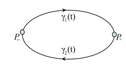
We consider an autonomous ordinary differential equation that admits a heteroclinic loop. The unperturbed heteroclinic loop consists of two degenerate heteroclinic orbits $ \gamma_1 $ and $ \gamma_2 $. We assume the variational equation along the degenerate heteroclinic orbit $ \gamma_i $ has $ {d_i}\left({{d_i} > 1, i = 1, 2} \right) $ linearly independent bounded solutions. Moreover, the splitting indices of the unperturbed heteroclinic orbits are $ s $ and $ -s $ $ (s\geq 0) $, respectively. In this paper, we study the persistence of the heteroclinic loop under periodic perturbation. Using the method of Lyapunov-Schmidt reduction and exponential dichotomies, we obtained the bifurcation function, which is defined from $ \mathbb{R}^{d_1+d_2+2} $ to $ \mathbb{R}^{d_1+d_2} $. Under some conditions, the perturbed system can have a heteroclinic loop near the unperturbed heteroclinic loop.

References

[1]	J. R. Guckenheimer, P. Holmes, Nonlinear Oscillations, Dynamical Systems, and Bifurcations of Vector Fields, Springer-Verlag, New York, 1983.
[2]	K. H. Alfsen, J. Fr$\phi$yland, Systematics of the Lorenz model at $\sigma = 10$, Phys. Scr., 31 (1985), 15–20. https://doi.org/10.1088/0031-8949/31/1/003 doi: 10.1088/0031-8949/31/1/003
[3]	C. Bonatti, L. J. Díaz, M. Viana, Dynamics Beyond Uniform Hyperbolicity: A Global Geometric and Probabilistic Perspective, Springer-Verlag, New York, 2005.
[4]	M. Han, J. Yang, A. Tarta, Y. Gao, Limit cycles near homoclinic and heteroclinic loops, J. Dyn. Differ. Equations, 20 (2008). https://doi.org/10.1007/s10884-008-9108-3
[5]	X. Sun, M. Han, J. Yang, Bifurcation of limit cycles from a heteroclinic loop with a cusp, Nonlinear Anal. Theory Methods Appl., 74 (2011), 2948–2965. https://doi.org/10.1016/j.na.2011.01.013 doi: 10.1016/j.na.2011.01.013
[6]	F. Chen, A. Oksasoglu, Q. Wang, Heteroclinic tangles in time-periodic equations, J. Differ. Equations, 254 (2013), 1137–1171. https://doi.org/10.1016/j.jde.2012.10.010 doi: 10.1016/j.jde.2012.10.010
[7]	I. S. Labouriau, A. A. P. Rodrigues, Periodic forcing of a heteroclinic network, J. Dyn. Differ. Equations, 2021 (2021). https://doi.org/10.1007/s10884-021-10054-w
[8]	I. S. Labouriau, A. A. P. Rodrigues, Bifurcations from an attracting heteroclinic cycle under periodic forcing, J. Differ. Equations, 269 (2020), 4137–4174. https://doi.org/10.1016/j.jde.2020.03.024 doi: 10.1016/j.jde.2020.03.024
[9]	S. N. Chow, B. Deng, D. Terman, The bifurcation of homoclinic and periodic orbits from two heteroclinic orbits, SIAM J. Math. Anal., 21 (1990), 179–204. https://doi.org/10.1137/0521010 doi: 10.1137/0521010
[10]	D. Zhu, Z. Xia, Bifurcations of heteroclinic loops, Sci. China Ser. A Math., 41 (1998), 837–848. https://doi.org/10.1007/BF02871667 doi: 10.1007/BF02871667
[11]	J. D. M. Rademacher, Homoclinic orbits near heteroclinic cycles with one equilibrium and one periodic orbit, J. Differ. Equations, 218 (2005), 390–443. https://doi.org/10.1016/j.jde.2005.03.016 doi: 10.1016/j.jde.2005.03.016
[12]	X. Lin, Using Melnikov's method to solve Shilnikov's problems, Proc. R. Soc. Edinburgh Sect. A Math., 116 (1990), 295–325. https://doi.org/10.1017/S0308210500031528 doi: 10.1017/S0308210500031528
[13]	F. Geng, T. Wang, X. Liu, Global bifurcations near a degenerate hetero-dimernsional cycle, J. Appl. Anal. Comput., 8 (2018), 123–151. https://doi.org/10.11948/2018.123 doi: 10.11948/2018.123
[14]	X. Liu, X. Wang, T. Wang, Nongeneric bifurcations near a nontransversal heterodimensional cycle, Chin. Ann. Math. Ser. B, 39 (2018), 111–128. https://doi.org/10.1007/s11401-018-1055-7 doi: 10.1007/s11401-018-1055-7
[15]	A. Vanderbauwhede, Bifurcation of degenerate homoclinics, Results Math., 21 (1992), 211–223. https://doi.org/10.1007/BF03323080 doi: 10.1007/BF03323080
[16]	S. N. Chow, J. K. Hale, Methods of Bifurcation Theory, Springer-Verlag, New York, 1982.
[17]	X. Lin, Lin's method, Scholarpedia, 3 (2008), 6972.
[18]	S. N. Chow, J. K. Hale, J. Mallet-Parret, An example of bifurcation to homoclinic orbits, J. Differ. Equations, 37 (1980), 551–573. https://doi.org/10.1016/0022-0396(80)90104-7 doi: 10.1016/0022-0396(80)90104-7
[19]	K. J. Palmer, Transversal heteroclinic points and Cherry's example of a nonintegrable Hamiltonian system, J. Differ. Equations, 65 (1986), 321–360. 10.1016/0022-0396(86)90023-9 doi: 10.1016/0022-0396(86)90023-9
[20]	J. K. Hale, X. Lin, Heteroclinic orbits for retarded functional differential equations, J. Differ. Equations, 65 (1986), 175–202. https://doi.org/10.1016/0022-0396(86)90032-X doi: 10.1016/0022-0396(86)90032-X
[21]	J. R. Gruendler, Homoclinic solutions for autonomous systems in arbitrary dimension, SIAM J. Math. Anal., 23 (1992), 702–721. https://doi.org/10.1137/0523036 doi: 10.1137/0523036
[22]	J. Gruendler, Homoclinic solutions for autonomous ordinary differential equations with nonautonomous perturbation, J. Differ. Equations, 122 (1995), 1–26. https://doi.org/10.1006/jdeq.1995.1136 doi: 10.1006/jdeq.1995.1136
[23]	R. J. Sacker, The splitting index for linear differential systems, J. Differ. Equations, 33 (1979), 368–405. https://doi.org/10.1016/0022-0396(79)90072-X doi: 10.1016/0022-0396(79)90072-X

Reader Comments

Your name:*

Email:*
© 2023 the Author(s), licensee AIMS Press. This is an open access article distributed under the terms of the Creative Commons Attribution License (http://creativecommons.org/licenses/by/4.0)