Multi-shockpeakons for the stochastic Degasperis-Procesi equation

Lynnyngs K. Arruda; Lynnyngs K. Arruda

doi:10.3934/era.2022117

Electronic Research Archive

2022, Volume 30, Issue 6: 2303-2320. doi: 10.3934/era.2022117

Previous Article Next Article

Research article

Multi-shockpeakons for the stochastic Degasperis-Procesi equation

Lynnyngs K. Arruda ^,

Departamento de Matemática, Universidade Federal de São Carlos. CP 676, 13565-905, São Carlos - SP, Brazil

Received: 14 October 2021 Revised: 09 January 2022 Accepted: 09 January 2022 Published: 21 April 2022

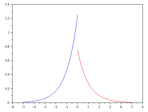
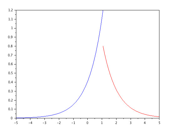
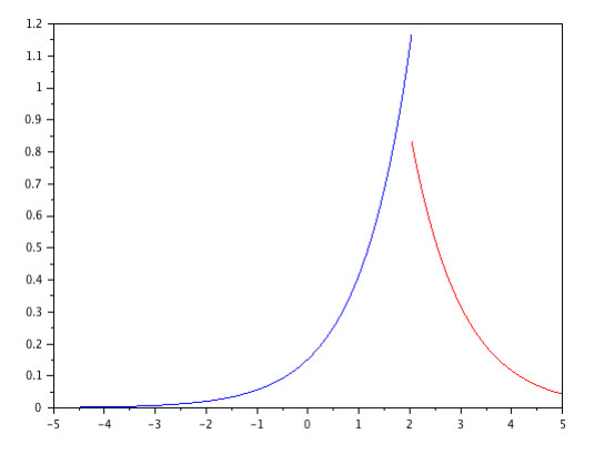
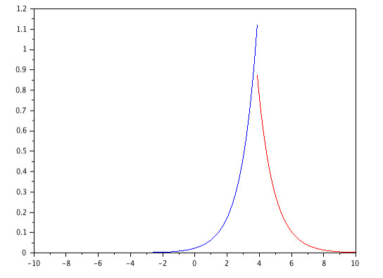
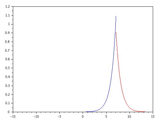
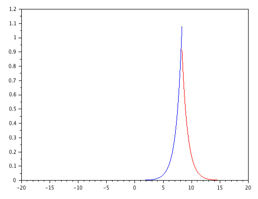
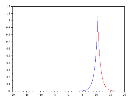
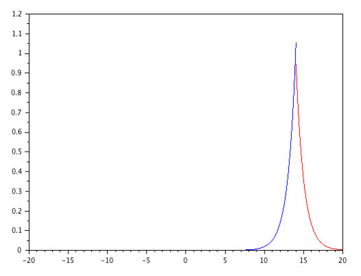
The deterministic Degasperis-Procesi equation admits weak multi-shockpeakon solutions of the form

$ u(x, t) = \sum\limits_{i = 1}^nm_i(t)e^{-|x-x_i(t)|}-\sum\limits_{i = 1}^ns_i(t){\rm sgn}(x-x_i(t))e^{-|x-x_i(t)|}, $

where $ {\rm sgn}(x) $ denotes the signum function with $ {\rm sgn}(0) = 0 $, if and only if the time-dependent parameters $ x_i(t) $ (positions), $ m_i(t) $ (momenta) and $ s_i(t) $ (shock strengths) satisfy a system of $ 3n $ ordinary differential equations. We prove that a stochastic perturbation of the Degasperis-Procesi equation also has weak multi-shockpeakon solutions if and only if the positions, momenta and shock strengths obey a system of $ 3n $ stochastic differential equations.
Citation: Lynnyngs K. Arruda. Multi-shockpeakons for the stochastic Degasperis-Procesi equation[J]. Electronic Research Archive, 2022, 30(6): 2303-2320. doi: 10.3934/era.2022117

Related Papers:

Abstract

The deterministic Degasperis-Procesi equation admits weak multi-shockpeakon solutions of the form

$ u(x, t) = \sum\limits_{i = 1}^nm_i(t)e^{-|x-x_i(t)|}-\sum\limits_{i = 1}^ns_i(t){\rm sgn}(x-x_i(t))e^{-|x-x_i(t)|}, $

where $ {\rm sgn}(x) $ denotes the signum function with $ {\rm sgn}(0) = 0 $, if and only if the time-dependent parameters $ x_i(t) $ (positions), $ m_i(t) $ (momenta) and $ s_i(t) $ (shock strengths) satisfy a system of $ 3n $ ordinary differential equations. We prove that a stochastic perturbation of the Degasperis-Procesi equation also has weak multi-shockpeakon solutions if and only if the positions, momenta and shock strengths obey a system of $ 3n $ stochastic differential equations.

References

[1]	L. K. Arruda, N. V. Chemetov, F. Cipriano, Solvability of the Stochastic Degasperis-Procesi Equation, J. Dyn. Differ. Equ., (2021), 1–20. https://doi.org/10.1007/s10884-021-10021-5 doi: 10.1007/s10884-021-10021-5
[2]	S. Hakkaev, I. D. Iliev, K. Kirchev, Stability of periodic travelling shallow-water waves determined by Newton' s equation, J. Phys. A: Math. Theor., 41 (2008), 085203. https://doi.org/10.1088/1751-8113/41/8/085203 doi: 10.1088/1751-8113/41/8/085203
[3]	R. Camassa, D. D. Holm, An integrable shallow water equation with peaked solitons, Phys. Rev. Lett., 71 (1993), 1661–1664. https://doi.org/10.1103/PhysRevLett.71.1661 doi: 10.1103/PhysRevLett.71.1661
[4]	A. Fokas, B. Fuchssteiner, Symplectic structures, their Backlund transformation and hereditary symmetries, Physica D, 4 (1982), 47–66. https://doi.org/10.1016/0362-546X(81)90025-0 doi: 10.1016/0362-546X(81)90025-0
[5]	J. Lenells, Classification of all travelling-wave solutions for some nonlinear dispersive equations, Phil. Trans. R. Soc. A, 365 (2007), 2291–2298. https://doi.org/10.1098/rsta.2007.2009 doi: 10.1098/rsta.2007.2009
[6]	T. M. Bendall, C. J. Cotter, D. D. Holm, Perspectives on the formation of peakons in the stochastic Camassa-Holm equation, Proc. R. Soc. A., 477 (2021), 20210224. https://doi.org/10.1098/rspa.2021.0224 doi: 10.1098/rspa.2021.0224
[7]	Y. Chen, H. Gao, B. Guo, Well-posedness for stochastic Camassa-Holm equation, J. Differ. Equ., 253 (2012), 2353–2379. https://doi.org/10.1016/j.jde.2012.06.023 doi: 10.1016/j.jde.2012.06.023
[8]	D. Crisan, D. D. Holm, Wave breaking for the stochastic Camassa-Holm equation, Physica D, 376 (2018), 138–143. https://doi.org/10.1016/j.physd.2018.02.004 doi: 10.1016/j.physd.2018.02.004
[9]	D. D. Holm, T. M. Tyranowski, Variational principles for stochastic soliton dynamics, Proc. Math. Phys. Eng. Sci., 472 (2016), 20150827. https://doi.org/10.1098/rspa.2015.0827 doi: 10.1098/rspa.2015.0827
[10]	G. Lv, J. Wei, G. Zou, The dependence on initial data of stochastic Camassa-Holm equation, Appl. Math. Lett., (2020), 106472. https://doi.org/10.1016/j.aml.2020.106472 doi: 10.1016/j.aml.2020.106472
[11]	X. Deng, A note on exact travelling wave solutions for the modified Camassa-Holm and Degasperis-Procesi equations, Appl. Math. Comput., 218 (2009), 2269–2276. https://doi.org/10.1016/j.amc.2011.07.044 doi: 10.1016/j.amc.2011.07.044
[12]	A. Darós, L. K. Arruda Saraiva de Paiva, The Modified Camassa-Holm Equation: Wave breaking, Classification of Traveling Waves and Explicit Elliptic Peakons, arXiv preprint, (2018), arXiv: 1809.02529.
[13]	H. R. Dullin, G. A. Gottwald, D. D. Holm, An integrable shallow water equation with linear and nonlinear dispersion, Phys. Rev. Lett., 87 (2001), 194501. https://doi.org/10.1103/PhysRevLett.87.194501 doi: 10.1103/PhysRevLett.87.194501
[14]	C. Rohde, H. Tang, On the stochastic Dullin-Gottwald-Holm equation: Global existence and wave-breaking phenomena, Nonlinear Differ. Equ. Appl., 28 (2021), 1–34. https://doi.org/10.1007/s00030-021-00676-w doi: 10.1007/s00030-021-00676-w
[15]	A. Degasperis, M. Procesi, Asymptotic integrability, in Symmetry and Perturbation Theory, (Rome, 1998), World Sci. Publishing, River Edge, NJ, (1999), 23–37.
[16]	G. M. Coclite, K. Karlsen, N. Risebro, Numerical schemes for computing discontinuous solutions of the Degasperis-Procesi equation, IMA J. Numer. Anal., 28 (2008), 80–105. https://doi.org/10.1093/imanum/drm003 doi: 10.1093/imanum/drm003
[17]	Z. Yin, On the Cauchy problem for an integrable equation with peakon solutions, Illinois J. Math., 47 (2003), 649–666. https://doi.org/10.1215/ijm/1258138186 doi: 10.1215/ijm/1258138186
[18]	H. Lundmark, Formation and dynamics of shock waves in the Degasperis-Procesi equation, J. Nonlinear Sci., 17 (2007), 169–198. https://doi.org/10.1007/s00332-006-0803-3 doi: 10.1007/s00332-006-0803-3
[19]	H. Lundmark, J. Szmigeilski, Multi-peakon solutions of the Degasperis-Procesi equation, Inverse Probl., 19 (2003), 1241–1245. https://doi.org/10.1088/0266-5611/19/6/001 doi: 10.1088/0266-5611/19/6/001
[20]	H. Lundmark, J. Szmigeilski, Degasperis-Procesi peakons and the discrete cubic string, Int. Math. Res. Papers, 2 (2005), 53–116. https://doi.org/10.1155/IMRP.2005.53 doi: 10.1155/IMRP.2005.53
[21]	A. Degasperis, D. D. Holm, A. N. W. Hone, A New Integrable Equation with Peakon Solutions, Theor. Math. Phys., 133 (2002), 1463–1474. https://doi.org/10.1023/A:1021186408422 doi: 10.1023/A:1021186408422
[22]	G. M. Coclite, K. H. Karlsen, On the well-posedness of the Degasperis-Procesi equation, J. Funct. Anal., 233 (2006), 60–91. https://doi.org/10.1016/j.jfa.2005.07.008 doi: 10.1016/j.jfa.2005.07.008
[23]	J. Escher, Y. Liu, Z. Yin, Shock waves and blow-up phenomena for the periodic Degasperis - Procesi equation, Indiana Univ. Math. J., 56 (2007), 87–117. https://doi.org/10.1512/iumj.2007.56.3040 doi: 10.1512/iumj.2007.56.3040
[24]	J. Szmigeilski, L. Zhou, Peakon-antipeakon interactions in the Degasperis-Procesi equation, in algebraic and geometric aspects of integrable systems and random matrices, Contemp. Math., 593 (2013), 83–107. https://doi.org/10.1090/conm/593/11873 doi: 10.1090/conm/593/11873
[25]	Y. Chen, H. Gao, Global existence for the stochastic Degasperis-Procesi equation, Discrete Contin. Dyn. Syst., 35 (2015), 5171–5184. https://doi.org/10.3934/dcds.2015.35.5171 doi: 10.3934/dcds.2015.35.5171
[26]	B. Perthame, Kinetic formulation of conservation laws, Oxford University Press, 2002.
[27]	H. A. Hoel, A numerical scheme using multi-shockpeakons to compute solutions of the Degasperis-Procesi equation, Electron. J. Differ. Equ., 2007 (2007), 1–22.

Reader Comments

Your name:*

Email:*
© 2022 the Author(s), licensee AIMS Press. This is an open access article distributed under the terms of the Creative Commons Attribution License (http://creativecommons.org/licenses/by/4.0)