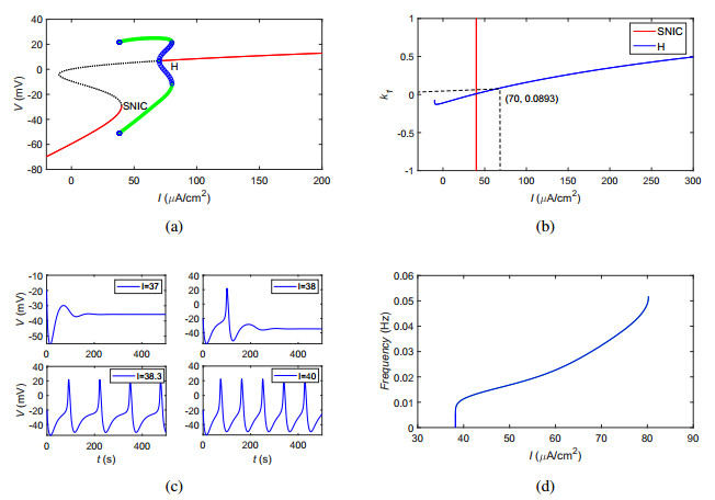
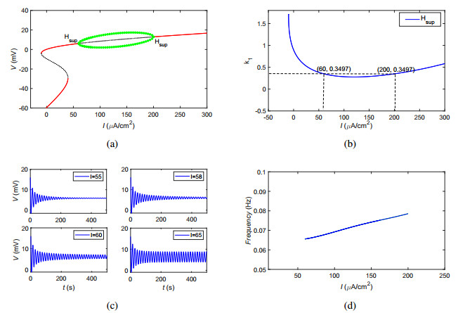
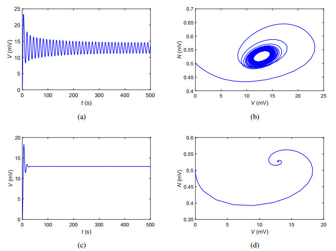
It is shown that many neurological diseases are caused by the changes of firing patterns induced by bifurcations. Therefore, the bifurcation control may provide a potential therapeutic method of these neurodegenerative diseases. In this paper, we investigate the Hopf bifurcation control of the Morris-Lecar (ML) model with Homoclinic (Hc) bifurcation type by introducing a dynamic state-feedback control. The results indicate that the linear term can change the ML model from Hc bifurcation type to SNIC bifurcation type without changing the firing patterns. The cooperation of linear and cubic term can transform the ML model from the Hc bifurcation type to the Hopf bifurcation type, resulting in the transformation of firing patterns from type I to type II. Besides, we utilize the Poincare Birkhoff (PB) normal form method to derive the analytical expression of the bifurcation stability index for the controlled ML model with Hc bifurcation type, and the results show that the cubic term can regulate the criticality of the Hopf bifurcation. Numerical simulation results are consistent with the theoretical analysis.
Citation: Qinghua Zhu, Meng Li, Fang Han. Hopf bifurcation control of the ML neuron model with Hc bifurcation type[J]. Electronic Research Archive, 2022, 30(2): 615-632. doi: 10.3934/era.2022032
It is shown that many neurological diseases are caused by the changes of firing patterns induced by bifurcations. Therefore, the bifurcation control may provide a potential therapeutic method of these neurodegenerative diseases. In this paper, we investigate the Hopf bifurcation control of the Morris-Lecar (ML) model with Homoclinic (Hc) bifurcation type by introducing a dynamic state-feedback control. The results indicate that the linear term can change the ML model from Hc bifurcation type to SNIC bifurcation type without changing the firing patterns. The cooperation of linear and cubic term can transform the ML model from the Hc bifurcation type to the Hopf bifurcation type, resulting in the transformation of firing patterns from type I to type II. Besides, we utilize the Poincare Birkhoff (PB) normal form method to derive the analytical expression of the bifurcation stability index for the controlled ML model with Hc bifurcation type, and the results show that the cubic term can regulate the criticality of the Hopf bifurcation. Numerical simulation results are consistent with the theoretical analysis.

| [1] | G. B. Ermentrout, D. H. Terman, Mathematical foundations of neuroscience, Springer-Verlag, New York, 2010. |
| [2] |
A. L. Hodgkin, A. F. Huxley, A quantitative description of membrane current and its application to conduction and excitation in nerve, J. Physiol., 117 (1952), 500–544. https://doi.org/10.1113/jphysiol.1952.sp004764 doi: 10.1113/jphysiol.1952.sp004764

|
| [3] |
R. FitzHugh, Impulses and physiological states in theoretical models of nerve membrane, Biophys. J., 1 (1961), 445466. https://doi.org/10.1016/s0006-3495(61)86902-6 doi: 10.1016/s0006-3495(61)86902-6
|
| [4] |
C. Morris, H. Lecar, Voltage oscillations in the barnacle giant muscle fiber, Biophys. J., 35 (1981), 193–213. https://doi.org/:10.1016/s0006-3495(81)84782-0 doi: 10.1016/s0006-3495(81)84782-0
|
| [5] |
J. L. Hindmarsh, R. M. Rose, A model of neuronal bursting using three coupled first order differential equations, Proc. R. Soc. Lond. Ser. B, 221 (1984), 87–102. https://doi.org/10.2307/35900 doi: 10.2307/35900
|
| [6] |
Q. Zheng, J. W. Shen, Turing instability induced by random network in FitzHugh-Nagumo model, Appl. Math. Comput., 381 (2020), 125304. https://doi.org/10.1016/j.amc.2020.125304 doi: 10.1016/j.amc.2020.125304
|
| [7] |
A. Mondal, R. K. Upadhyay, J. Ma, B. K. Yadav, S. K. Sharma, A. Mondal, Bifurcation analysis and diverse firing activities of a modified excitable neuron model, Cogn. Neurodyn., 13 (2019), 393–407. https://doi.org/10.1007/s11571-019-09526-z doi: 10.1007/s11571-019-09526-z
|
| [8] |
M. K. Wouapi, B. H. Fotsin, E. B. M. Ngouonkadi, F. F. Kemwoue, Z. T. Njitacke, Complex bifurcation analysis and synchronization optimal control for Hindmarsh-Rose neuron model under magnetic flow effect, Cogn. Neurodyn., 15 (2021), 315–347. https://doi.org/10.1007/s11571-020-09606-5 doi: 10.1007/s11571-020-09606-5
|
| [9] | J. Milton, P. Jung, Brain defibrillators: synopsis, problems and future directions. In: Epilepsy as a Dynamic Disease, Springer, Berlin Heidelberg, 2003. |
| [10] |
Y. Xie, L. Chen, Y. Kang, K. Aihara, Controlling the onset of Hopf bifurcation in the Hodgkin-Huxley model, Phys. Rev. E., 77 (2008), 061921. https://doi.org/10.1103/PhysRevE.77.061921 doi: 10.1103/PhysRevE.77.061921
|
| [11] |
L. Nguyen and K. Hong, Hopf bifurcation control via a dynamic state-feedback control, Phys. Lett. A, 376 (2012), 442–446. https://doi.org/10.1016/j.physleta.2011.11.057 doi: 10.1016/j.physleta.2011.11.057
|
| [12] |
Y. Xie, Change in types of neuronal excitebility via bifurcation control, Chin. Q. Mech., 31 (2010), 58–63. https://doi.org/10.1103/PhysRevE.77.021917 doi: 10.1103/PhysRevE.77.021917
|
| [13] |
D. J. Schulz, Plasticity and stability in neuronal output via changes in intrinsic excitability: it's what's inside that counts, J. Exp. Biol., 209 (2006), 4821–4827. https://doi.org/10.1242/jeb.02567 doi: 10.1242/jeb.02567
|
| [14] |
G. R. Chen, J. L. Moiola, H. O. Wang, Bifurcation Control: Theories, Methods, and Applications, Int. J. Bifurc. Chaos, 10 (2000), 511–548. https://doi.org/10.1142/S0218127400000360 doi: 10.1142/S0218127400000360
|
| [15] |
X. F. Liao, S. W. Li, K. W. Wong, Hopf bifurcation on a twoneuron system with distributed delays: a frequency domain approach, Nonlinear Dyn., 31 (2003), 299–326. https://doi.org/10.1023/A:1022928118143 doi: 10.1023/A:1022928118143
|
| [16] |
P. Yu, G. R. Chen, Hopf bifurcation control using nonlinear feedback with polynomial functions, Int. J. Bifurc. Chaos, 14 (2004), 1683–1704. https://doi.org/10.1142/S0218127404010291 doi: 10.1142/S0218127404010291
|
| [17] |
J. Jiang, Y. L. Song, Delay-induced Bogdanov-Takens bifurcation in a Leslie-Gower predator-prey model with nonmonotonic functional response, Commun. Nonlinear. Sci. Numer. Simul., 19 (2014), 2454–2465. https://doi.org/10.1016/j.cnsns.2013.11.020 doi: 10.1016/j.cnsns.2013.11.020
|
| [18] |
M. Xiao, D. Ho, J. Cao, Time-delayed feedback control of dynamical small-world networks at Hopf bifurcation, Nonlinear Dyn., 58 (2009), 319–344. https://doi.org/10.1007/s11071-009-9485-0 doi: 10.1007/s11071-009-9485-0
|
| [19] |
C. L. Huang, W. Sun, Z. G. Zheng, J. H. Lu, S. H. Chen, Hopf bifurcation control of the M-L neuron model with type I, Nonlinear Dyn., 87 (2017), 755–766. https://doi.org/10.1007/s11071-016-3073-x doi: 10.1007/s11071-016-3073-x
|
| [20] |
L. H. Nguyen, K. S. Hong, Hopf bifurcation control via a dynamic state-feedback control, Phys. Lett. A, 376 (2012), 442–446. https://doi.org/10.1016/j.physleta.2011.11.057 doi: 10.1016/j.physleta.2011.11.057
|
| [21] | J. Rinzel, G. B. Ermentrout, Analysis of Neural Excitability and Oscillations, In: Koch, C. and Segev, I., Eds., Methods in Neuronal Modeling: From Synapses to Networks, MIT Press, Cambridge, 1989,135–169. |
| [22] | E. M. Izhikevich, Dynamical Systems in Neuroscience, Cambridge, Massachusetts: MIT Press, 2007. |
| [23] |
W. Liu, Criterion of Hopf bifurcations without using eigenvalues, J. Math. Anal. Appl., 182 (1994), 250–256. https://doi.org/10.1006/jmaa.1994.1079 doi: 10.1006/jmaa.1994.1079
|
Figures(7) / Tables(1)
Qinghua Zhu, Meng Li, Fang Han. Hopf bifurcation control of the ML neuron model with Hc bifurcation type[J]. Electronic Research Archive, 2022, 30(2): 615-632. doi: 10.3934/era.2022032


 DownLoad: