Path-connectedness in global bifurcation theory

J. F. Toland; J. F. Toland

doi:10.3934/era.2021079

Electronic Research Archive

2021, Volume 29, Issue 6: 4199-4213. doi: 10.3934/era.2021079

Previous Article Next Article

Special Issues

Path-connectedness in global bifurcation theory

J. F. Toland

Department of Mathematical Sciences, University of Bath, Bath BA2 7AY, UK

Received: 01 April 2021 Revised: 01 August 2021 Published: 08 October 2021
Primary: 47J15, 58E07, 35B32; Secondary: 54F15

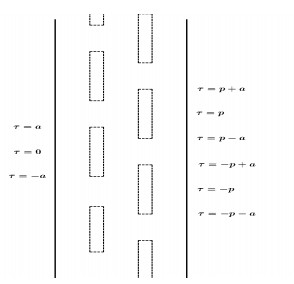
A celebrated result in bifurcation theory is that, when the operators involved are compact, global connected sets of non-trivial solutions bifurcate from trivial solutions at non-zero eigenvalues of odd algebraic multiplicity of the linearized problem. This paper presents a simple example in which the hypotheses of the global bifurcation theorem are satisfied, yet all the path-connected components of the connected sets that bifurcate are singletons. Another example shows that even when the operators are everywhere infinitely differentiable and classical bifurcation occurs locally at a simple eigenvalue, the global continua may not be path-connected away from the bifurcation point. A third example shows that the non-trivial solutions which bifurcate at non-zero eigenvalues, irrespective of multiplicity when the problem has gradient structure, may not be connected and may not contain any paths except singletons.
- Global bifurcation,
- point-set topology,
- path-connectedness,
- hereditarily indecomposable continua,
- topological degree,
- variational methods
Citation: J. F. Toland. Path-connectedness in global bifurcation theory[J]. Electronic Research Archive, 2021, 29(6): 4199-4213. doi: 10.3934/era.2021079

Related Papers:

Abstract

A celebrated result in bifurcation theory is that, when the operators involved are compact, global connected sets of non-trivial solutions bifurcate from trivial solutions at non-zero eigenvalues of odd algebraic multiplicity of the linearized problem. This paper presents a simple example in which the hypotheses of the global bifurcation theorem are satisfied, yet all the path-connected components of the connected sets that bifurcate are singletons. Another example shows that even when the operators are everywhere infinitely differentiable and classical bifurcation occurs locally at a simple eigenvalue, the global continua may not be path-connected away from the bifurcation point. A third example shows that the non-trivial solutions which bifurcate at non-zero eigenvalues, irrespective of multiplicity when the problem has gradient structure, may not be connected and may not contain any paths except singletons.

References

[1]	Concerning hereditarily indecomposable continua. Pacific J. Math. (1951) 1: 43-51.
[2]	Snake-like continua. Duke Math. J. (1951) 18: 653-663.
[3]	Die Lösung der Verzweigungsgleichungen für nichtlineare Eigenwertprobleme. Math. Zeit. (1972) 127: 105-126.
[4]	(2003) Analytic Theory of Global Bifurcation,. Princeton and Oxford: Princeton University Press.
[5]	Chainable continua and indecomposability. Pacific J. Math. (1959) 9: 653-659.
[6]	Bifurcation from simple eigenvalues. J. Funct. Anal. (1971) 8: 321-340.
[7]	Bifurcation theory for analytic operators. Proc. Lond. Math. Soc. (1973) 26: 359-384.
[8]	Global structure of the solutions of non-linear real analytic eigenvalue problems. Proc. Lond. Math. Soc. (1973) 27: 747-765.
[9]	Bifurcation from simple eigenvalues and eigenvalues of geometric multiplicity one. Bull. Lond. Math. Soc. (2002) 34: 533-538.
[10]	J. J. Duistermaat and J. A. C. Kolk, Multidimensional Real Analysis I., Cambridge Studies in Advanced Mathematics 86. Cambridge University Press, Cambridge, 2004. doi: 10.1017/CBO9780511616716
[11]	N. Dunford and J. T. Schwartz, Linear Operators, Part Ⅰ: General Theory, , With the assistance of W. G. Bade and R. G. Bartle. Pure and Applied Mathematics, Vol. 7 Interscience Publishers, Inc., New York; Interscience Publishers, Ltd., London, 1958.
[12]	The pseudo-circle is unique,. Trans. Amer. Math. Soc. (1970) 149: 45-64.
[13]	A brief historical view of continuum theory. Topology Appl. (2006) 153: 1530-1539.
[14]	Un continu dont tout sous-continu est indécomposable. Fund. Math. (1922) 3: 247-286.
[15]	On a topological method in the problem of eigenfunctions of nonlinear operators. Dokl. Akad. Nauk SSSR (N.S.) (1950) 74: 5-7.
[16]	Some problems in nonlinear analysis. Amer. Math. Soc. Trans. Ser. (1958) 10: 345-409.
[17]	. A. Krasnolsel'skii, Topological Methods in the Theory of Nonlinear Eigenvalue Problems, Pergamon Press, Oxford, 1963. (Original in Russian: Topologicheskiye Metody v Teorii Nelineinykh Integral'nykh Uravnenii., Gostekhteoretizdat, Moscow, 1956.)
[18]	Some global results for nonlinear eigenvalue problems. J. Funct. Anal. (1971) 7: 487-513.
[19]	Some aspects of nonlinear eigenvalue problems. Rocky Mountain J. Math. (1973) 3: 161-202.
[20]	H. L. Royden, Real Analysis, Third Edition, McMillan, New York, 1988.
[21]	Global bifurcation for $k$-set contractions without multiplicity assumptions. Quart. J. Math. Oxford Ser. (1976) 27: 199-216.
[22]	M. M. Vainberg, Variational Methods for the Study of Nonlinear Operators, With a chapter on Newton's method by L. V. Kantorovich and G. P. Akilov. Translated and supplemented by Amiel Feinstein Holden-Day, Inc., San Francisco, Calif.-London-Amsterdam, 1964.

Reader Comments

your name:*

Email:*
© 2021 the Author(s), licensee AIMS Press. This is an open access article distributed under the terms of the Creative Commons Attribution License (http://creativecommons.org/licenses/by/4.0)