Traveling wave solution for a diffusion SEIR epidemic model with self-protection and treatment

Hai-Feng Huo; Shi-Ke Hu; Hong Xiang; Hai-Feng Huo; Shi-Ke Hu; Hong Xiang

doi:10.3934/era.2020118

Electronic Research Archive

2021, Volume 29, Issue 3: 2325-2358. doi: 10.3934/era.2020118

Previous Article Next Article

Traveling wave solution for a diffusion SEIR epidemic model with self-protection and treatment

Department of Applied Mathematics, Lanzhou University of Technology, Lanzhou, Gansu 730050, China

Received: 01 August 2020 Revised: 01 October 2020 Published: 24 November 2020
Primary: 35C07, 35B40, 35K57; Secondary: 92D30

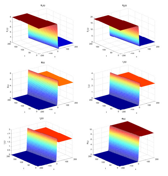
A reaction-diffusion SEIR model, including the self-protection for susceptible individuals, treatments for infectious individuals and constant recruitment, is introduced. The existence of traveling wave solution, which is determined by the basic reproduction number $ R_0 $ and wave speed $ c, $ is firstly proved as $ R_0>1 $ and $ c\geq c^* $ via the Schauder fixed point theorem, where $ c^* $ is minimal wave speed. Asymptotic behavior of traveling wave solution at infinity is also proved by applying the Lyapunov functional. Furthermore, when $ R_0\leq1 $ or $ R_0>1 $ with $ c\in(0,\ c^*), $ we derive the non-existence of traveling wave solution with utilizing two-sides Laplace transform. We take advantage of numerical simulations to indicate the existence of traveling wave, and show that self-protection and treatment can reduce the spread speed at last.
- Self-protection,
- treatment,
- Schauder fixed point theorem,
- Lyapunov functional,
- two-sides Laplace transform
Citation: Hai-Feng Huo, Shi-Ke Hu, Hong Xiang. Traveling wave solution for a diffusion SEIR epidemic model with self-protection and treatment[J]. Electronic Research Archive, 2021, 29(3): 2325-2358. doi: 10.3934/era.2020118

Related Papers:

Abstract

A reaction-diffusion SEIR model, including the self-protection for susceptible individuals, treatments for infectious individuals and constant recruitment, is introduced. The existence of traveling wave solution, which is determined by the basic reproduction number $ R_0 $ and wave speed $ c, $ is firstly proved as $ R_0>1 $ and $ c\geq c^* $ via the Schauder fixed point theorem, where $ c^* $ is minimal wave speed. Asymptotic behavior of traveling wave solution at infinity is also proved by applying the Lyapunov functional. Furthermore, when $ R_0\leq1 $ or $ R_0>1 $ with $ c\in(0,\ c^*), $ we derive the non-existence of traveling wave solution with utilizing two-sides Laplace transform. We take advantage of numerical simulations to indicate the existence of traveling wave, and show that self-protection and treatment can reduce the spread speed at last.

References

[1]	Traveling waves in spatial SIRS models. J. Dynam. Differential Equations (2014) 26: 143-164.
[2]	Harnack's inequality for cooperative weakly coupled elliptic systems: Harnack's inequality. Comm. Partial Differential Equations (1999) 24: 1555-1571.
[3]	Travelling wave solutions in multigroup age-structured epidemic models. Arch. Ration. Mech. Anal. (2010) 195: 311-331.
[4]	Traveling waves for monotone semiflows with weak compactness. SIAM J. Math. Anal. (2014) 46: 3678-3704.
[5]	A. Friedman, Partial Differential Equations of Parabolic Type, Prentice-Hall, Englewood Cliffs, 2008.
[6]	D. Gilbarg and N. S. Trudinger, Elliptic Partial Differential Equations of Second Order, Springer, 2015.
[7]	Hyperbolic travelling fronts. Proc. Edinburgh Math. Soc. (1988) 31: 89-97.
[8]	Travelling fronts for correlated random walks. Canad. Appl. Math. Quart. (1994) 2: 27-43.
[9]	Stability and bifurcation for an SEIS epidemic model with the impact of media. Phys. A (2018) 490: 702-720.
[10]	Dynamics for an SIRS epidemic model with infection age and relapse on a scale-free network. J. Franklin Inst. (2019) 356: 7411-7443.
[11]	J. S. Jia, X. Lu, Y. Yuan, G. Xu, J. Jia and N. A. Christakis, Population flow drives spatio-temporal distribution of COVID-19 in China, Nature, 1–5.
[12]	S.-L. Jing, H.-F. Huo and H. Xiang, Modeling the effects of meteorological factors and unreported cases on seasonal influenza outbreaks in Gansu province, China, Bull. Math. Biol., 82 (2020), Paper No. 73, 36 pp. doi: 10.1007/s11538-020-00747-6
[13]	Effect of non-pharmaceutical interventions to contain COVID-19 in China. Nature (2020) 585: 410-413.
[14]	Traveling waves for a nonlocal dispersal SIR model with delay and external supplies. Appl. Math. Comput. (2014) 247: 723-740.
[15]	Global stability of an epidemic model with latent stage and vaccination. Nonlinear Anal. Real World Appl. (2011) 12: 2163-2173.
[16]	Asymptotic speeds of spread and traveling waves for monotone semiflows with applications. Comm. Pure Appl. Math. (2007) 60: 1-40.
[17]	Effective containment explains subexponential growth in recent confirmed COVID-19 cases in China. Science (2020) 368: 742-746.
[18]	J. D. Murray, Mathematical Biology, Springer, 1989. doi: 10.1007/978-3-662-08539-4
[19]	M. H. Protter and H. F. Weinberger, Maximum Principles in Differential Equations, Springer, 2012.
[20]	L. Rass and J. Radcliffe, Spatial Deterministic Epidemics, American Mathematical Society, 2003. doi: 10.1090/surv/102
[21]	Large-scale spatial-transmission models of infectious disease. Science (2007) 316: 1298-1301.
[22]	Global Hopf bifurcation of a delayed equation describing the lag effect of media impact on the spread of infectious disease. J. Math. Biol. (2018) 76: 1249-1267.
[23]	Analysis of an epidemic system with two response delays in media impact function. Bull. Math. Biol. (2019) 81: 1582-1612.
[24]	Reproduction numbers and sub-threshold endemic equilibria for compartmental models of disease transmission. Math. Biosci. (2002) 180: 29-48.
[25]	J.-B. Wang and C. Wu, Forced waves and gap formations for a Lotka–Volterra competition model with nonlocal dispersal and shifting habitats, Nonlinear Analysis: Real World Applications, 58 (2021), 103208, 19 pp. doi: 10.1016/j.nonrwa.2020.103208
[26]	Traveling waves of the spread of avian influenza. Proc. Amer. Math. Soc. (2012) 140: 3931-3946.
[27]	Traveling waves in a nonlocal anisotropic dispersal Kermack-Mckendrick epidemic model. Discrete Contin. Dyn. Syst. Ser. B (2013) 18: 1969-1993.
[28]	Minimal wave speed for a class of non-cooperative reaction–diffusion systems of three equations. J. Differential Equations (2017) 262: 4724-4770.
[29]	Existence of traveling wave solutions for influenza model with treatment. J. Math. Anal. Appl. (2014) 419: 469-495.
[30]	Minimal wave speed for a class of non-cooperative diffusion–reaction system. J. Differential Equations (2016) 260: 2763-2791.
[31]	Traveling wave fronts in a diffusive epidemic model with multiple parallel infectious stages. IMA J. Appl. Math. (2016) 81: 795-823.
[32]	Traveling wave solutions in a two-group epidemic model with latent period. Nonlinearity (2017) 30: 1287-1325.
[33]	Traveling wave solutions in a two-group SIR epidemic model with constant recruitment. J. Math. Biol. (2018) 77: 1871-1915.

Reader Comments

your name:*

Email:*
© 2021 the Author(s), licensee AIMS Press. This is an open access article distributed under the terms of the Creative Commons Attribution License (http://creativecommons.org/licenses/by/4.0)