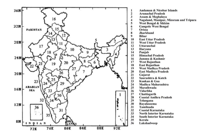
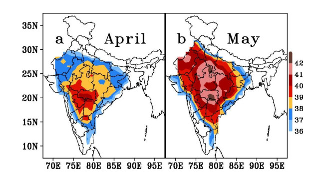
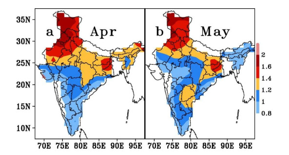
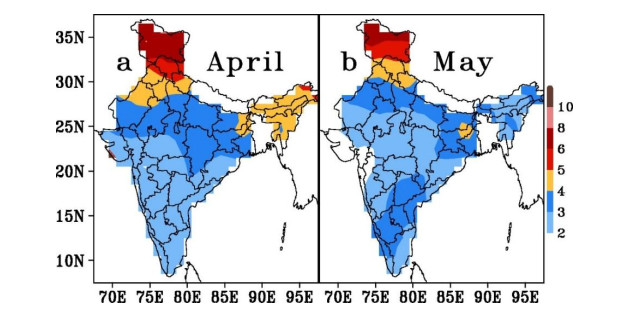
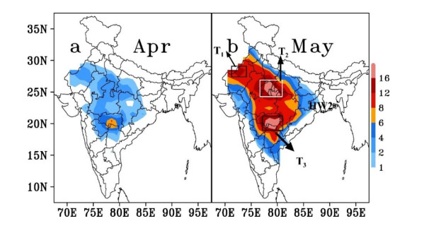
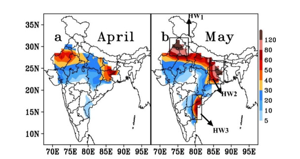
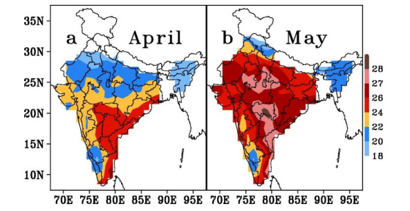
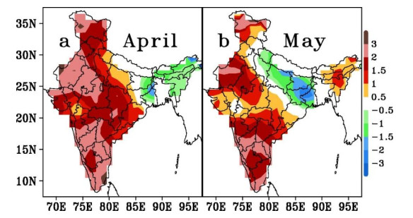
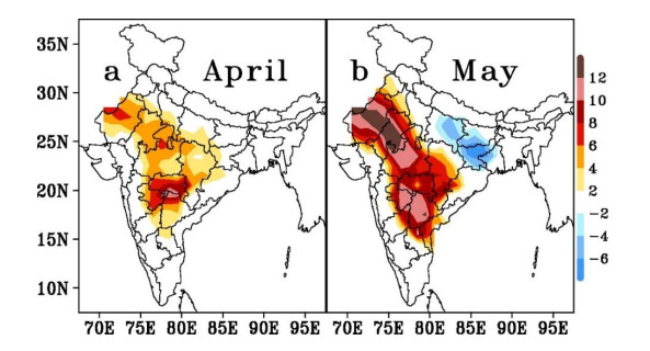
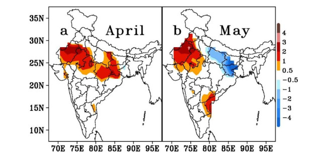
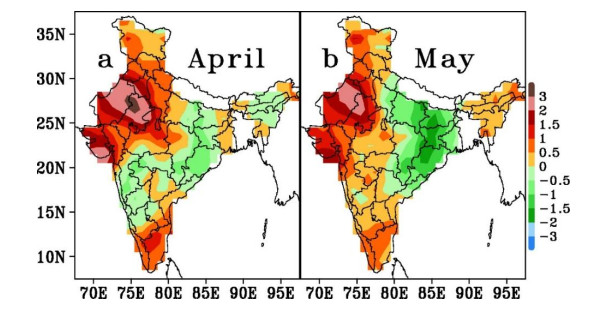
The climate of a place has a decisive role in human adaptations. Man's health, adaptability, behavioural patterns, food, shelter, and clothing are mainly influenced by the temperatures of the area. Hence, a study is undertaken to analyse the spatial distribution, frequency, and trend in the heat waves over the country. The statistical characteristics of heat waves over India are addressed in this study. Gridded daily temperature data sets for the period 1951–2019 were used to compute the arithmetic mean (AM), standard deviation (SD), coefficient of variation (CV), and trends of monthly maximum temperature. The number of heat wave days were identified using the criteria given by India Meteorological Department (IMD) i.e., a heat wave is recognized when the daily normal maximum temperature of a station is less than or equal to (greater than) 40 ℃ than it will be considered as a heat wave if the daily maximum temperature exceeds the daily normal maximum temperature by 5 ℃ (4 ℃). The analysis was confined to the two summer months of April and May only. The spatial distribution of the AM shows higher values during May, and the core hot region with temperatures exceeding 40 ℃ lies over central India extending towards the northwest. The SD distribution shows higher values over the northeast of central India decreasing towards the southwest. The CV distribution shows higher values over the north decreasing toward the south. Higher numbers of heat waves are observed during May and the number is higher over Andhra Pradesh and south Telangana regions of southeast India. This study concludes that a moderate hot region experiences a higher number of heat wave days over India.
Citation: N. Naveena, G. Ch. Satyanarayana, A. Dharma Raju, K Sivasankara Rao, N. Umakanth. Spatial and statistical characteristics of heat waves impacting India[J]. AIMS Environmental Science, 2021, 8(2): 117-134. doi: 10.3934/environsci.2021009
The climate of a place has a decisive role in human adaptations. Man's health, adaptability, behavioural patterns, food, shelter, and clothing are mainly influenced by the temperatures of the area. Hence, a study is undertaken to analyse the spatial distribution, frequency, and trend in the heat waves over the country. The statistical characteristics of heat waves over India are addressed in this study. Gridded daily temperature data sets for the period 1951–2019 were used to compute the arithmetic mean (AM), standard deviation (SD), coefficient of variation (CV), and trends of monthly maximum temperature. The number of heat wave days were identified using the criteria given by India Meteorological Department (IMD) i.e., a heat wave is recognized when the daily normal maximum temperature of a station is less than or equal to (greater than) 40 ℃ than it will be considered as a heat wave if the daily maximum temperature exceeds the daily normal maximum temperature by 5 ℃ (4 ℃). The analysis was confined to the two summer months of April and May only. The spatial distribution of the AM shows higher values during May, and the core hot region with temperatures exceeding 40 ℃ lies over central India extending towards the northwest. The SD distribution shows higher values over the northeast of central India decreasing towards the southwest. The CV distribution shows higher values over the north decreasing toward the south. Higher numbers of heat waves are observed during May and the number is higher over Andhra Pradesh and south Telangana regions of southeast India. This study concludes that a moderate hot region experiences a higher number of heat wave days over India.

| [1] |
Coumou D, Rahmstorf S (2012) A decade of weather extremes. Nat Climate Change 2: 491–496. doi: 10.1038/nclimate1452

|
| [2] | IPCC, 2013: Summary for policymakers. Climate Change 2013: The Physical Science Basis, T. F. Stocker et al., Eds., Cambridge University Press, 1–30. |
| [3] | Perkins SE, Alexander LV, Nairn J.R (2012). Increasing frequency, intensity and duration of observed global heatwaves and warm spells. Geop hys Res Lett 39: L20714. |
| [4] | Perkins SE (2015) A review on the scientific understanding of heatwaves-Their measurement, driving mechanisms, and changes at the global scale. Atmos. Res 164–165: 242–267. |
| [5] |
Mora C, Mora C, Dousset B, et al (2017) Global risk of deadly heat. Nat Climate Change 7: 501–506. doi: 10.1038/nclimate3322
|
| [6] |
Nissan H, K Burkart, EC dePerez, et al. (2017) Defining and predicting heat waves in Bangladesh. J Appl Meteor Climatol 56: 2653–2670. doi: 10.1175/JAMC-D-17-0035.1
|
| [7] | IPCC, 2007. Climate Change 2007: Impacts, Adaptation and Vulnerability. Contribution of Working Group II to the IPCC Fourth Assessment Report. Cambridge University Press: Cambridge. |
| [8] |
Poumadere M, Mays C, Le Mer S, et al. (2006) The 2003 heat wave in France: Dangerous climate here and now. Risk Anal 25: 1483–1494. doi: 10.1111/j.1539-6924.2005.00694.x
|
| [9] |
Sheridan SC, Kalkstein LS (2004) Progress in heat watch warning system technology. B Am Meteorol Soc 85: 1931–1941. doi: 10.1175/BAMS-85-12-1931
|
| [10] | Srivastava harinarain, BN Diwan, SK Dikshit, et al. (1993) Decadal trends in climate over India. Mausam 43: 7–20. |
| [11] | Pramanik SK, Jagannathan P (1954) Climatic change in India: II. Temperature. Indian J Meteorol Geophys 5: 1–19. |
| [12] |
Hingane LS, Rupa Kumar K, Ramana Murthy Bh V (1985) Long-term trends of surface air temperature in India. Int J Climatol 5: 521–528. doi: 10.1002/joc.3370050505
|
| [13] | Simister J, Cary C (2004) Thermal stress in the U.S.A.: effects on violence and on employee behaviour. Stress and Health (International Society for the Investigation of Stress) 21: 3–15. |
| [14] | Bell M, Giannini A, Grover E, et al. (2003) Climate Impacts. IRI Climate Digest (The Earth Institute). Retrieved 28 July 2006. |
| [15] |
Satyanarayana GC, Dodla DV (2020) Phenology of heat waves over India. Atmos Res 245: 105078. doi: 10.1016/j.atmosres.2020.105078
|
| [16] |
Filleul L, Cassadou S, Medina S, et al. (2006) The relation between temperature, ozone, and mortality in nine French cities during the heat wave of 2003. Env Health Persp 14: 1344–1347. doi: 10.1289/ehp.8328
|
| [17] | Grize L, Huss A, Thommen O, et al. (2005) Heat wave 2003 and mortality in Switzerland. Swiss Med Weekly 135: 200–205. |
| [18] |
Rusticucci M, Vargas W (2002) Cold and warm events over Argentina and their relationship with the ENSO phases: risk evaluation analysis. Int J Climatol 22: 467–483. doi: 10.1002/joc.743
|
| [19] | Gutowski WJ, GC Hegerl, GJ Holland, et al. (2008) Causes of Observed Changes in Extremes and Projections of Future Changes in Weather and Climate Extremes in a Changing Climate. Regions of Focus: North America, Hawaii, Caribbean, and U.S. Pacific Islands. T.R. Karl, Meehl G.A, Miller C.D, Hassol S.J, Waple A.M, and Murray, W.L, (eds.). A Report by the U.S. Climate Change Science Program and the Subcommittee on Global Change Research, Washington, DC. |
| [20] | NDMA (National Disaster Management Authority) 2016. Guidelines for Preparation of Action Plan–Prevention and Management of Heat Wave, National Disaster Management Authority, Government of India, 13. |
| [21] |
Mani A, Chacko O (1973) Solar radiation climate of India. Sol Energy 14: 139–156. doi: 10.1016/0038-092X(73)90030-3
|
| [22] |
Ross RS, Krishnamurti TN, Pattnaik Sandeep, et al. (2018) Decadal surface temperature trends in India based on a new high resolution data set. Sci Rep 8: 7452. doi: 10.1038/s41598-018-25347-2
|
| [23] | Dodla VB, Satyanarayana CG, Desamsetti S (2017) Analysis and prediction of a catastrophic Indian coastal heat wave of 2015. Nat Hazards. 87: 395–414. |
| [24] |
Yadav RK (2016). On the relationship between Iran surface temperature and north-West India summer monsoon rainfall. Int J Climatol 36: 4425–4438. doi: 10.1002/joc.4648
|
| [25] |
Fink AH, Brucher T, Kruger A, et al. (2004) The 2003 European summer heatwaves and drought—synoptic diagnosis and impacts. Weather 59: 209–216. doi: 10.1256/wea.73.04
|
| [26] |
Schar C, Jendritzky G (2004) Hot news from summer 2003. Nature 432: 559–560. doi: 10.1038/432559a
|
| [27] |
Kunkel KE, TR Karl DR, Easterling K, et al. (2013) Probable maximum precipitation and climate change. Geophys Res Lett 40: 1402–1408. doi: 10.1002/grl.50334
|
| [28] |
Palecki MA, Changnon SA, Kunkel KE (2001) The nature and impacts of the July 1999 heat wave in the midwestern United States: learning from the lessons of 1995. B Am Meteorol Soc 82: 1353–1367. doi: 10.1175/1520-0477(2001)082<1353:TNAIOT>2.3.CO;2
|
| [29] | Steffen W, Hughes L, Perkins S (2014) Heat waves: hotter, longer, more often. Climate Council of Australia Limited. http://www.climatecouncil.org.au/uploads/9901f6614a2cac7b2b888f55b4dff9cc.pdf |
| [30] |
Peterson TC, Heim RR Jr, Hirsch R, et al. (2013) Monitoring and understanding changes in heat waves, cold waves, floods and droughts in the United States, state of knowledge. Bull Am Meteorol Soc 94: 821–834. doi: 10.1175/BAMS-D-12-00066.1
|
| [31] |
Garcia-Herrera R, Diaz J, Trigo RM, et al. (2010) A review of the European summer heat wave of 2003. Crit Rev Environ Sci Technol 40: 267–306. doi: 10.1080/10643380802238137
|
| [32] | Desai DS (1999) Heat wave conditions during March to June for the year 1972, 1979 and 1987 and their comparison with year 1990–1995. Mausam 50: 211–218. |
| [33] | Raghavan K (1966) A climatological study of sever heat wave in India. Indian J Met Geophys 17: 581–586. |
| [34] | Subbaramayya I, Suryanaryana Rao DA (1976) Heat wave and cold wave days in different states in India. Indian J Met Hydrol Geophys 27: 436. |
| [35] | Pai DS, Smitha AN, Ramatathan AN (2013) Long term climatology and trendsof heatwaves over India during the recent 50 years (1961-2010). Mausam 64: 585–604. |
| [36] | Chaudhary V (2015) Minister of public safety and emergency preparedness, Canada. ONCA 678: 108. |
| [37] | Bedekar VC, Dekate MV, Banerjee AK (1974) Heat and cold wave in India. India Meteorological Department, Forecasting Manual FMU Rep. No. IV-6. http://www.imdpune.gov.in/Weather/Reports/glossary.pdf |
| [38] | Srivastava A, Rajeevan M, Kshirsagar S (2009) Development of a high resolution daily gridded temperature data set (1969–2005) for the Indian region. Atmos Sci Lett 10: 249–254. |
| [39] | Naveena N, Satyanarayana GC, Rao DVB, et al. (2020) An accentuated "hot blob" over Vidarbha, India, during the pre-monsoon season. Nat Hazards. 105: 1359–1373. |
| [40] | Menon PA (1989). Our Weather. (National Book Trust, India). |
Figures(11) / Tables(2)

N. Naveena, G. Ch. Satyanarayana, A. Dharma Raju, K Sivasankara Rao, N. Umakanth. Spatial and statistical characteristics of heat waves impacting India[J]. AIMS Environmental Science, 2021, 8(2): 117-134. doi: 10.3934/environsci.2021009


 DownLoad: