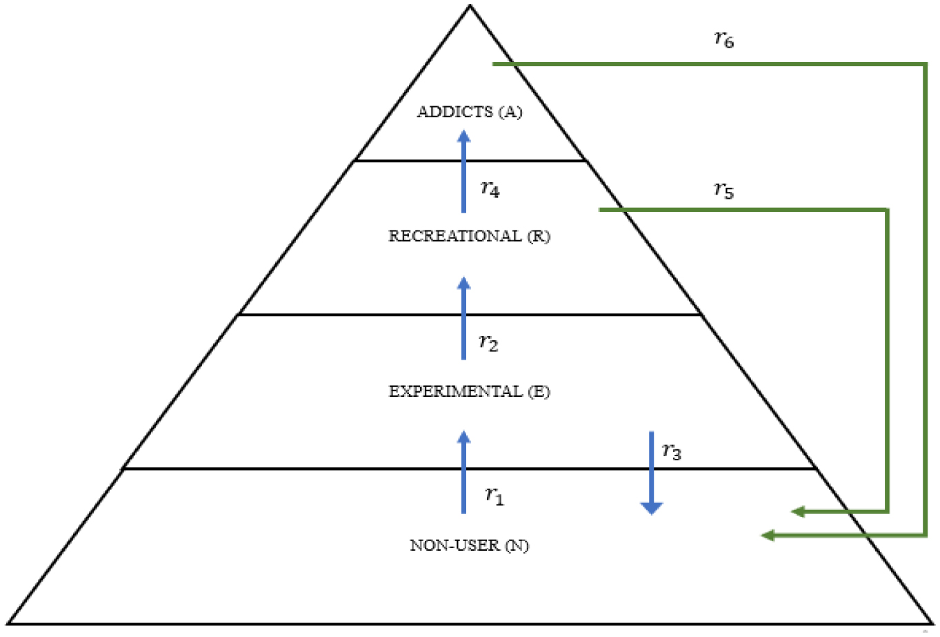
The aim of the current study is to reduce marijuana use among the general population. Because marijuana is an illegal narcotic with numerous negative health effects, it continues to pose a severe threat to public health in emerging nations. In this article, a modified mathematical model of the non-users, experimental users, recreational users, and addict's (NERA) model for marijuana consumption is established by incorporating a new compartment that represents the individuals who are being moved to jail by police intervention. The overall population of humans is divided into five main components: the non-smoker's compartment, experimental smoker's compartment, recreational smoker's compartment, addicted smoker's compartment, and prisoner's compartment. The novelty of this work is to modify the NERA model for marijuana consumption and validate the modified model. Furthermore, with the help of sensitivity analysis, control strategies for marijuana consumption in the population are addressed. The invariant region and the basic reproductive number (R0) are those parts that are needed for the validation of the proposed model. For the numerical simulation of the given model, the 4th-order Runge Kutta method will be used with the help of MATLAB to examine how the control strategies will play a role in marijuana consumption.
Citation: Atta Ullah, Hamzah Sakidin, Shehza Gul, Kamal Shah, Yaman Hamed, Maggie Aphane, Thabet Abdeljawad. Sensitivity analysis-based control strategies of a mathematical model for reducing marijuana smoking[J]. AIMS Bioengineering, 2023, 10(4): 491-510. doi: 10.3934/bioeng.2023028
The aim of the current study is to reduce marijuana use among the general population. Because marijuana is an illegal narcotic with numerous negative health effects, it continues to pose a severe threat to public health in emerging nations. In this article, a modified mathematical model of the non-users, experimental users, recreational users, and addict's (NERA) model for marijuana consumption is established by incorporating a new compartment that represents the individuals who are being moved to jail by police intervention. The overall population of humans is divided into five main components: the non-smoker's compartment, experimental smoker's compartment, recreational smoker's compartment, addicted smoker's compartment, and prisoner's compartment. The novelty of this work is to modify the NERA model for marijuana consumption and validate the modified model. Furthermore, with the help of sensitivity analysis, control strategies for marijuana consumption in the population are addressed. The invariant region and the basic reproductive number (R0) are those parts that are needed for the validation of the proposed model. For the numerical simulation of the given model, the 4th-order Runge Kutta method will be used with the help of MATLAB to examine how the control strategies will play a role in marijuana consumption.

| [1] | Algahtani OJ, Zeb A, Zaman G, et al. (2015) Mathematical study of smoking model by incorporating campaign class. Wulfenia 22: 205-216. |
| [2] |
Leong DP, Teo KK, Rangarajan S, et al. (2018) World Population Prospects 2019. Department of Economic and Social Affairs Population Dynamics. New York (NY): United Nations; 2019 ( |
| [3] |
Fligiel SEG, Roth MD, Kleerup EC, et al. (1997) Tracheobronchial histopathology in habitual smokers of cocaine, marijuana, and/or tobacco. Chest 112: 319-326. https://doi.org/10.1378/chest.112.2.319 
|
| [4] |
BALDWIN GC, Tashkin DP, Buckley DM, et al. (1997) Marijuana and cocaine impair alveolar macrophage function and cytokine production. Am J Respir Crit Care Med 156: 1606-1613. https://doi.org/10.1164/ajrccm.156.5.9704146
|
| [5] |
Shay AH, Choi R, Whittaker K, et al. (2003) Impairment of antimicrobial activity and nitric oxide production in alveolar macrophages from smokers of marijuana and cocaine. J Infect Dis 187: 700-704. https://doi.org/10.1086/368370
|
| [6] |
Naz H, Dumrongpokaphan T, Sitthiwirattham T, et al. (2023) A numerical scheme for fractional order mortgage model of economics. Results Appl Math 18: 100367. https://doi.org/10.1016/j.rinam.2023.100367
|
| [7] | Alrabaiah H, Ullah Z, Ahmad I, et al. Iterative investigation of korteweg–de vries equation using ab derivative in caputo sense (2023). https://doi.org/10.1142/s0218348x23400959 |
| [8] |
Moore THM, Zammit S, Lingford-Hughes A, et al. (2007) Cannabis use and risk of psychotic or affective mental health outcomes: a systematic review. Lancet 370: 319-328. https://doi.org/10.1016/s0140-6736(07)61162-3
|
| [9] |
Vozoris NT, Zhu J, Ryan CM, et al. (2022) Cannabis use and risks of respiratory and all-cause morbidity and mortality: a population-based, data-linkage, cohort study. BMJ Open Respir Res 9: e001216. https://doi.org/10.1136/bmjresp-2022-001216
|
| [10] | Tashkin DP, Coulson AH, Clark VA, et al. (1987) Respiratory symptoms and lung function in habitual heavy smokers of marijuana alone, smokers of marijuana and tobacco, smokers of tobacco alone, and nonsmokers. Am Rev Respir Dis 135: 209-216. https://doi.org/10.1378/chest.78.5.699 |
| [11] | Polen MR, Sidney S, Tekawa IS, et al. (1993) Health care use by frequent marijuana smokers who do not smoke tobacco. West J Med 158: 596. https://doi.org/10.1007/978-1-4615-1907-2_99 |
| [12] | Merz F (2018) United nations office on drugs and crime: world drug report 2017. 2017. SIRIUS-Zeitschr Strateg Anal 2: 85-86. https://doi.org/10.1515/sirius-2018-0016 |
| [13] |
Degenhardt L, Charlson F, Ferrari A, et al. (2018) The global burden of disease attributable to alcohol and drug use in 195 countries and territories, 1990–2016: a systematic analysis for the global burden of disease study 2016. Lancet Psychiatry 5: 987-1012. https://doi.org/10.1016/s2215-0366(18)30337-7
|
| [14] | Al Juboori R, Subramaniam DS, Hinyard L (2022) Understanding the role of adult mental health and substance abuse in perpetrating violent acts: In the presence of unmet needs for mental health services. Int J Ment Health Addiction 21: 1-9. https://doi.org/10.1007/s11469-022-00778-1 |
| [15] |
Lee J, Thrul J (2021) Trends in opioid misuse by cigarette smoking status among US adolescents: Results from national survey on drug use and health 2015–2018. Prev Med 153: 106829. https://doi.org/10.1016/j.ypmed.2021.106829
|
| [16] |
Testai FD, Gorelick PB, Aparicio HJ, et al. (2022) Use of marijuana: effect on brain health: a scientific statement from the American Heart Association. Stroke 53: e176-e187. https://doi.org/10.1161/str.0000000000000396
|
| [17] |
Beutler JA, Marderosian AH (1978) Chemotaxonomy of Cannabis I. Crossbreeding between Cannabis sativa and C. ruderalis, with analysis of cannabinoid content. Econ Bot 32: 387-394. https://doi.org/10.1007/bf02907934
|
| [18] |
Di Forti M, Morgan C, Dazzan P, et al. (2009) High-potency cannabis and the risk of psychosis. Br J Psychiatry 195: 488-491. https://doi.org/10.1192/bjp.bp.109.064220
|
| [19] | Mousavi SE, Bozorgian A (2020) Investigation the kinetics of CO2 hydrate formation in the water system+ CTAB+ TBAF+ ZnO. Int J New Chem 7: 195-219. https://doi.org/10.33945/sami/ecc.2020.4.10 |
| [20] |
Ellis RJ (2009) Smoked medicinal cannabis for neuropathic pain in HIV: a randomized, crossover clinical trial. Neuropsychopharmacology 34: 672-680. https://doi.org/10.1038/npp.2008.120
|
| [21] |
Russo E (2001) Cannabinoids in pain management: Study was bound to conclude that cannabinoids had limited efficacy. BMJ 323: 1249-1250. https://doi.org/10.1136/bmj.323.7323.1249
|
| [22] |
Russo EB (2008) Cannabinoids in the management of difficult to treat pain. Ther Clin Risk Manag 4: 245-259. https://doi.org/10.2147/tcrm.s1928
|
| [23] |
Cascini F, Aiello C, Di Tanna GL (2012) Increasing delta-9-tetrahydrocannabinol (Delta-9-THC) content in herbal cannabis over time: systematic review and meta-analysis. Curr Drug Abuse Rev 5: 32-40. https://doi.org/10.2174/1874473711205010032
|
| [24] | Savaki HE, Cunha J, Carlini EA, et al. (1976) Pharmacological activity of three fractions obtained by smoking cannabis through a water pipe. Bull Narc 28: 49-56. https://doi.org/10.1007/978-3-642-51624-5_39 |
| [25] | Samimi A, Zarinabadi S, Bozorgian A (2021) Optimization of corrosion information in oil and gas wells using electrochemical experiments. Int J New Chem 8: 149-163. https://doi.org/10.33945/sami/jcr.2020.2.5 |
| [26] |
Izadi M, Yüzbaşı Ş, Ansari KJ (2021) Application of Vieta–Lucas series to solve a class of multi-pantograph delay differential equations with singularity. Symmetry 13: 2370. https://doi.org/10.3390/sym13122370
|
| [27] |
Tashkin DP, Gliederer F, Rose J, et al. (1991) Tar, CO and Δ9-THC delivery from the 1st and 2nd halves of a marijuana cigarette. Pharmacol Biochem Behav 40: 657-661. https://doi.org/10.1016/0091-3057(91)90378-f
|
| [28] |
Aldington S, Williams M, Nowitz M, et al. (2007) Effects of cannabis on pulmonary structure, function and symptoms. Thorax 62: 1058-1063. https://doi.org/10.1136/thx.2006.077081
|
| [29] |
Bloom JW, Kaltenborn WT, Paoletti P, et al. (1987) Respiratory effects of non-tobacco cigarettes. Br Med J (Clin Res Ed) 295: 1516-1518. https://doi.org/10.1136/bmj.295.6612.1516
|
| [30] | Sadr MB, Bozorgian A (2021) An overview of gas overflow in gaseous hydrates. J Chem Rev 3: 66-82. https://doi.org/10.22034/jcr.2021.118870 |
| [31] |
Cruickshank EK (1976) Physical assessment of 30 chronic cannabis users and 30 matched controls. Ann N Y Acad Sci 282: 162-167. https://doi.org/10.1111/j.1749-6632.1976.tb49895.x
|
| [32] |
Tashkin DP, Simmons MS, Sherrill DL, et al. (1997) Heavy habitual marijuana smoking does not cause an accelerated decline in FEV1 with age. Am J Respir Crit Care Med 155: 141-148. https://doi.org/10.1164/ajrccm.155.1.9001303
|
| [33] | Tashkin DP, Reiss S, Shapiro BJ, et al. (1977) Bronchial effects of aerosolized Δ9-tetrahydrocannabinol in healthy and asthmatic subjects. Am Rev Respir Dis 115: 57-65. https://doi.org/10.1007/978-1-4613-4286-1_8 |
| [34] |
Din A, Li Y, Liu Q (2020) Viral dynamics and control of hepatitis B virus (HBV) using an epidemic model. Alexandria Eng J 59: 667-679. https://doi.org/10.1016/j.aej.2020.01.034
|
| [35] |
McNulty W, Usmani OS (2014) Techniques of assessing small airways dysfunction. Eur Clin Respir J 1: 25898. https://doi.org/10.3402/ecrj.v1.25898
|
| [36] |
Roth MD, Arora A, Barsky SH, et al. (1998) Airway inflammation in young marijuana and tobacco smokers. Am J Respir Crit Care Med 157: 928-937. https://doi.org/10.1164/ajrccm.157.3.9701026
|
| [37] | Bozorgian A (2021) Exergy analysis for evaluation of energy consumptions in hydrocarbon plants. Int J New Chem 8: 329-344. https://doi.org/10.22034/ijnc.2020.123715.1105 |
| [38] | US Department of Health and Human Services.The benefits of smoking cessation. A report of the surgeon general (DHHS publication no. CDC 90-8416) (1990) . |
| [39] |
Khan H, Alzabut J, Shah A, et al. (2023) On fractal-fractional waterborne disease model: A study on theoretical and numerical aspects of solutions via simulations. Fractals 2023: 2340055. https://doi.org/10.1142/s0218348x23400558
|
| [40] |
Khan H, Ahmed S, Alzabut J, et al. (2023) A generalized coupled system of fractional differential equations with application to finite time sliding mode control for Leukemia therapy. Chaos Solitons Fractals 174: 113901. https://doi.org/10.1016/j.chaos.2023.113901
|
| [41] | Bozorgian A (2020) Investigation of hydrate formation phenomenon and hydrate inhibitors. J Eng Ind Res 1: 99-110. https://doi.org/10.22034/ijnc.2020.123715.1105 |
| [42] |
Din A, Li Y, Khan T, et al. (2020) Mathematical analysis of spread and control of the novel corona virus (COVID-19) in China. Chaos Solitons Fractals 141: 110286. https://doi.org/10.1016/j.chaos.2020.110286
|
| [43] |
Tashkin DP (2015) The respiratory health benefits of quitting cannabis use. Eur Respir Soc 46: 1-4. https://doi.org/10.1183/09031936.00034515
|
| [44] | Bozorgian A, Ghanavati B (2020) Removal of copper II from industrial effluent with beta zeolite nanocryst. https://doi.org/10.22034/pcbr.2022.328704.1213 |
| [45] |
Ahmed S, Azar AT, Tounsi M (2022) Design of adaptive fractional-order fixed-time sliding mode control for robotic manipulators. Entropy 24: 1838. https://doi.org/https://doi.org/10.3390/e24121838
|
| [46] | Rabipour S, Abdulkareem Mahmood E, Afsharkhas M (2022) Medicinal use of marijuana and its impacts on respiratory system. J Chem Lett 3: 86-94. https://doi.org/10.22034/jchemlett.2022.347365.1072 |
| [47] |
Biehl JR, Burnham EL (2015) Cannabis smoking in 2015: a concern for lung health?. Chest 148: 596-606. https://doi.org/10.1378/chest.15-0447
|
| [48] |
Ryan SA, Ammerman SD, O'Connor ME, et al. (2018) Marijuana use during pregnancy and breastfeeding: implications for neonatal and childhood outcomes. Pediatrics 142: e20181889. https://doi.org/10.1542/peds.2018-1889
|
| [49] |
Dauhoo M, Korimboccus B, Issack S (2013) On the dynamics of illicit drug consumption in a given population. IMA J Appl Math 78: 432-448. https://doi.org/10.1093/imamat/hxr058
|
| [50] | Ginoux JM, Naeck R, Ruhomally YB, et al. (2019) Chaos in a predator–prey-based mathematical model for illicit drug consumption. Appl Math Comput 347: 502-513. https://doi.org/10.1016/j.amc.2018.10.089 |
| [51] | Ullah A, Sakidin H, Gul S, et al. (2023) Sensitivity analysis-based validation of the modified NERA model for improved performance. J Adv Res Appl Sci Eng Technol 32: 1-11. https://doi.org/10.37934/araset.32.3.111 |
| [52] |
Zamir M, Zaman G, Alshomrani AS (2016) Sensitivity analysis and optimal control of anthroponotic cutaneous leishmania. PloS one 11: e0160513. https://doi.org/10.1371/journal.pone.0160513
|
| [53] |
Zamir M, Abdeljawad T, Nadeem F, et al. (2021) An optimal control analysis of a COVID-19 model. Alexandria Eng J 60: 2875-2884. https://doi.org/10.1016/j.aej.2021.01.022
|
| [54] |
Liu P, Din A, Zarin R (2022) Numerical dynamics and fractional modeling of hepatitis B virus model with non-singular and non-local kernels. Results Phys 39: 105757. https://doi.org/10.1016/j.rinp.2022.105757
|
| [55] |
Zamir M, Zaman G, Alshomrani AS (2017) Control strategies and sensitivity analysis of anthroponotic visceral leishmaniasis model. J Biol Dyn 11: 323-338. https://doi.org/10.1080/17513758.2017.1339835
|
| [56] | Zamir M, Sultana R, Ali R, et al. (2015) Study on the threshold condition for infection of visceral leishmaniasis. Sindh Univ Res J 47: 619-622. |
| [57] |
Liu P, Huang X, Zarin R, et al. (2023) Modeling and numerical analysis of a fractional order model for dual variants of SARS-CoV-2. Alexandria Eng J 65: 427-442. https://doi.org/10.1016/j.aej.2022.10.025
|
| [58] |
Zamir M, Nadeem F, Alqudah MA, et al. (2022) Future implications of covid-19 through mathematical modeling. Results Phys 33: 105097. https://doi.org/10.1016/j.rinp.2021.105097
|
| [59] |
Madhusudanan V, Srinivas MN, Murthy BSN, et al. (2023) The influence of time delay and Gaussian white noise on the dynamics of tobacco smoking model. Chaos Solitons Fractals 173: 113616. https://doi.org/10.1016/j.chaos.2023.113616
|
| [60] |
Bushnaq S, Shah K, Tahir S, et al. (2022) Computation of numerical solutions to variable order fractional differential equations by using non-orthogonal basis. AIMS Math 7: 10917-10938. https://doi.org/10.3934/math.2022610
|
| [61] | Guo X, Guo Y, Zhao Z, et al. (2022) Computing R0 of dynamic models by a definition-based method. Infect Dis Model 7: 196-210. https://doi.org/10.1016/j.idm.2022.05.004 |
| [62] | Van den Driessche P (2017) Reproduction numbers of infectious disease models. Infect Dis Model 2: 288-303. https://doi.org/10.1016/j.idm.2017.06.002 |
| [63] |
Rodrigues HS, Monteiro MTT, Torres DFM (2013) Sensitivity analysis in a dengue epidemiological model. Conference Papers in Mathematics 2013: 1-7. https://doi.org/10.1155/2013/721406
|
| [64] | Ahmad N, Charan S, Singh VP (2015) Study of numerical accuracy of Runge-Kutta second, third and fourth order method. Int J Comput Math Sci 4: 111-118. |
| [65] | Islam MA (2015) Accurate solutions of initial value problems for ordinary differential equations with the fourth order Runge Kutta method. J Math Res 7: 41. https://doi.org/10.5539/jmr.v7n3p41 |
| [66] | Aida M (2022) Fourth-order runge-kutta method for solving applications of system of first-order ordinary differential equations. Enhanced Knowl Sci Technol 2: 517-526. https://doi.org/10.1007/s40995-017-0258-1 |


Figures(6) / Tables(3)

Atta Ullah, Hamzah Sakidin, Shehza Gul, Kamal Shah, Yaman Hamed, Maggie Aphane, Thabet Abdeljawad. Sensitivity analysis-based control strategies of a mathematical model for reducing marijuana smoking[J]. AIMS Bioengineering, 2023, 10(4): 491-510. doi: 10.3934/bioeng.2023028


 DownLoad: