Citation: Xu Guo. 2023: Annual Report 2022, AIMS Bioengineering, 10(1): 62-66. doi: 10.3934/bioeng.2023006

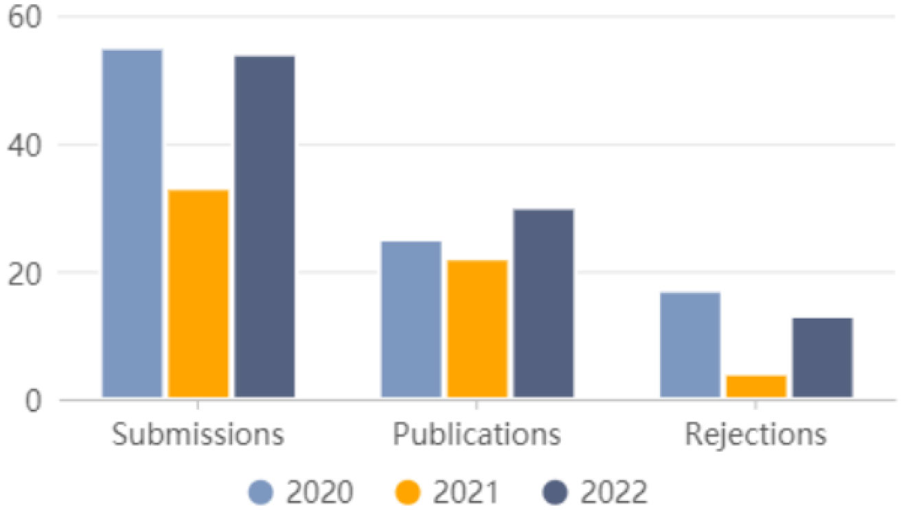
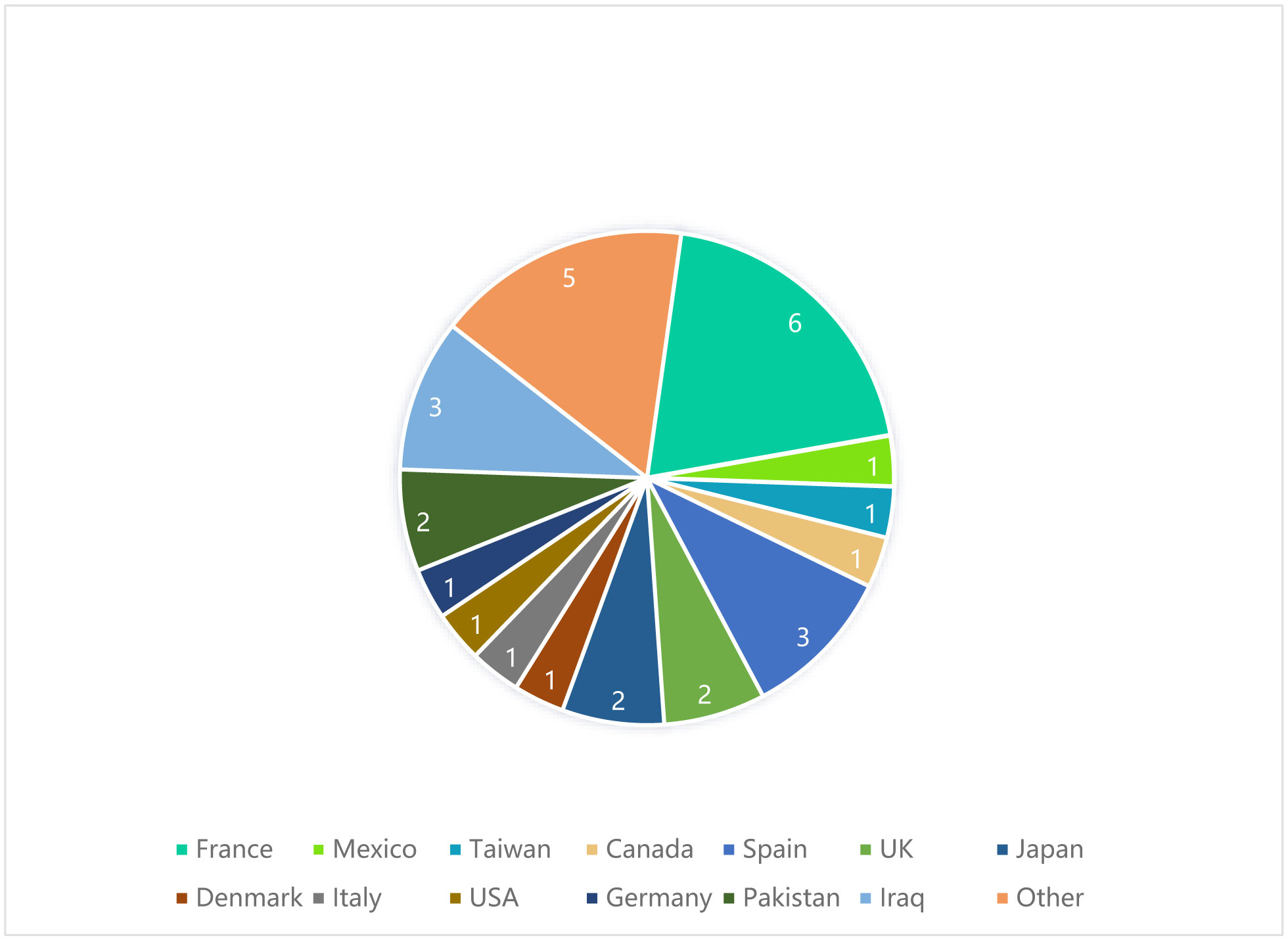
Figures(2) / Tables(1)


 DownLoad: