Sulcal pits of the superior temporal sulcus in schizophrenia patients with auditory verbal hallucinations

Baptiste Lerosier; Gregory Simon; Sylvain Takerkart; Guillaume Auzias; Sonia Dollfus; Baptiste Lerosier; Gregory Simon; Sylvain Takerkart; Guillaume Auzias; Sonia Dollfus

doi:10.3934/Neuroscience.2024002

AIMS Neuroscience

2024, Volume 11, Issue 1: 25-38. doi: 10.3934/Neuroscience.2024002

Previous Article Next Article

Research article Topical Sections

Sulcal pits of the superior temporal sulcus in schizophrenia patients with auditory verbal hallucinations

1.
Normandie Univ, UNICAEN, ISTS, EA 7466, 14000 Caen, France
2.
Aix Marseille Univ, CNRS, INT, Institut de Neurosciences de la Timone, Marseille, France
3.
CHU de Caen, Service de Psychiatrie, 14000 Caen, France
4.
Normandie Univ, UNICAEN, UFR santé, 14000 Caen, France
5.
Fédération Hospitalo-Universitaire (FHU-A²M²P), Normandie Univ, UNICAEN, UFR santé, 14000 Caen, France

Received: 27 October 2023 Revised: 16 January 2024 Accepted: 24 January 2024 Published: 31 January 2024

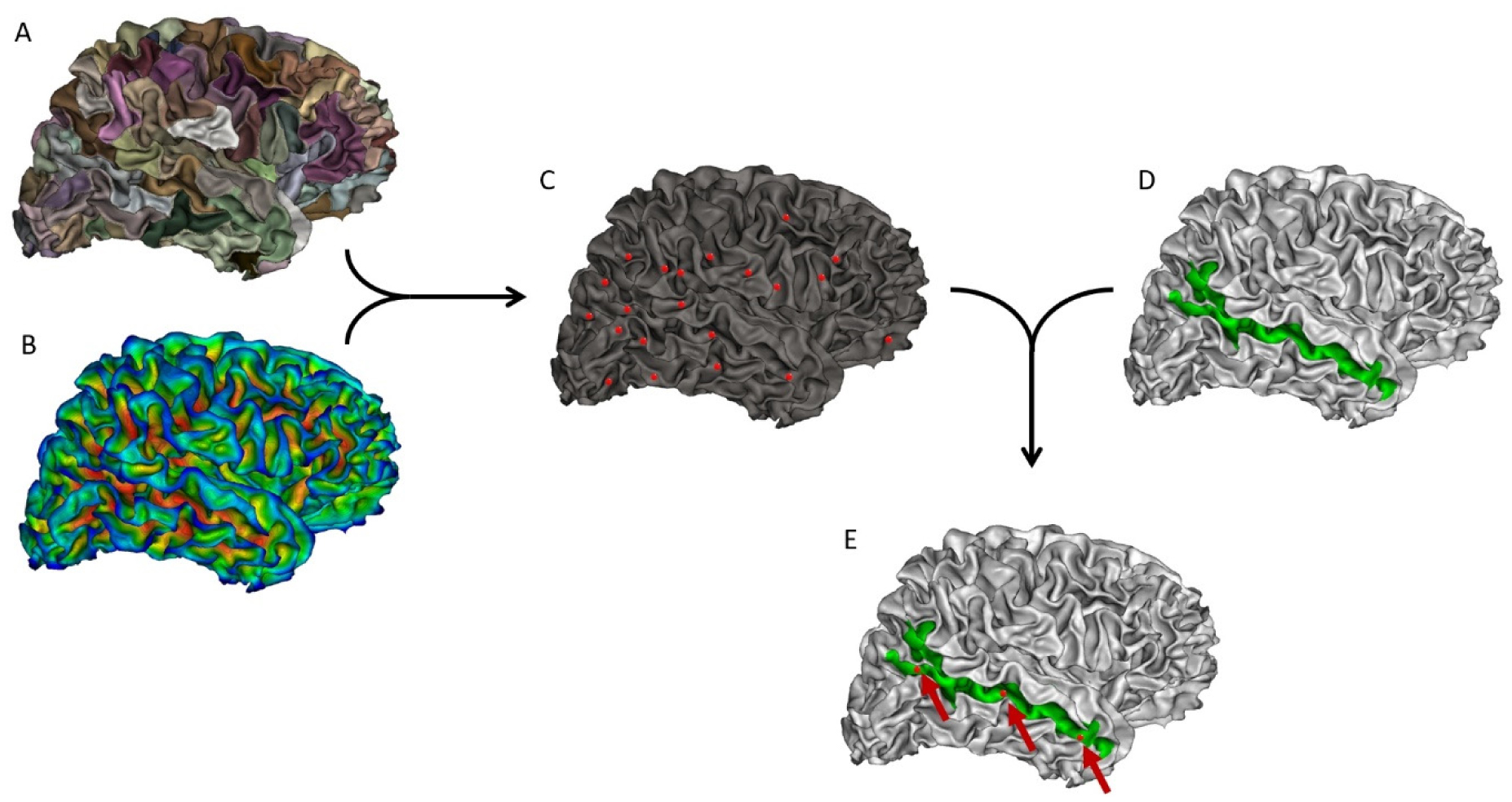
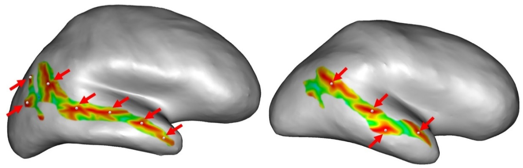
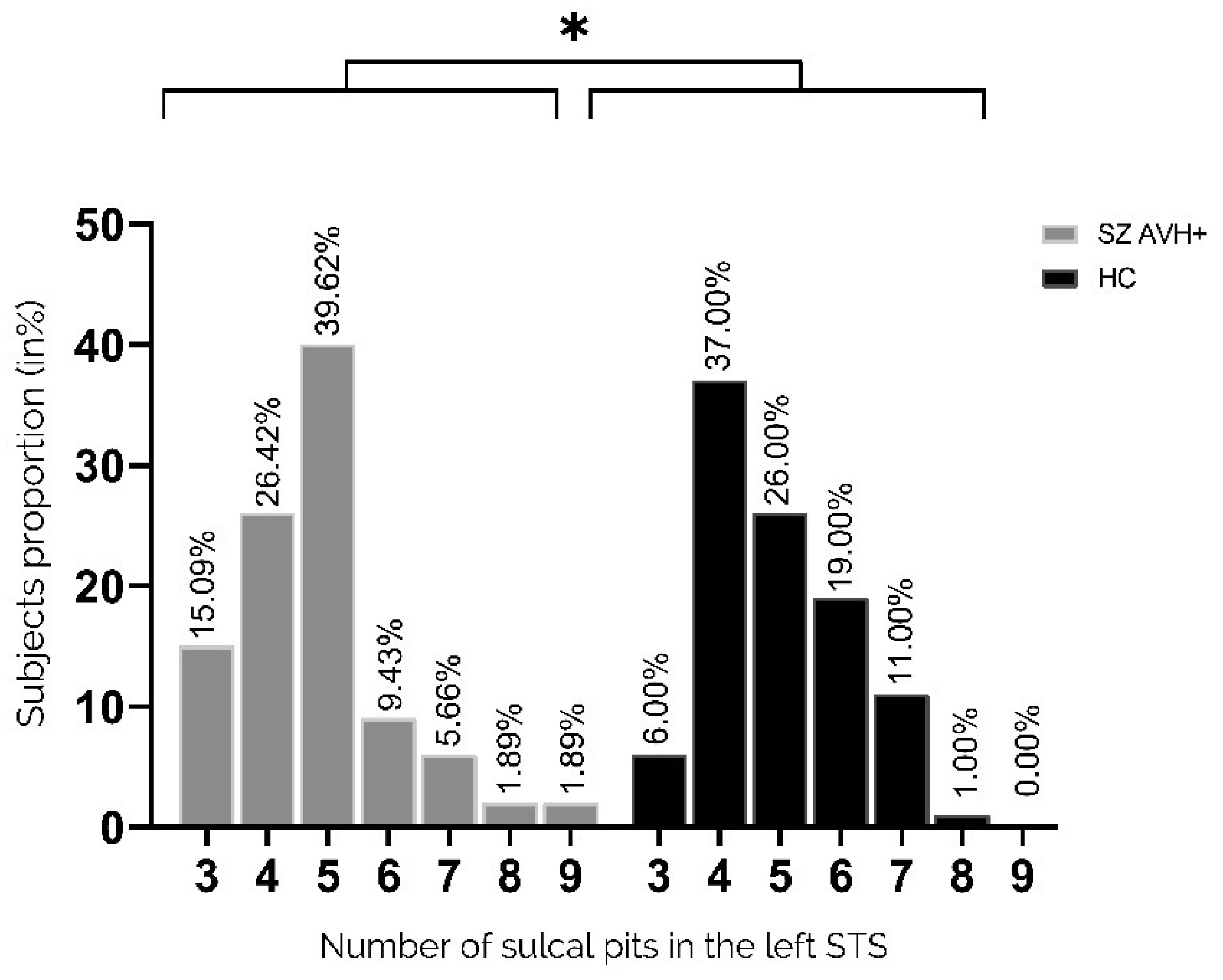
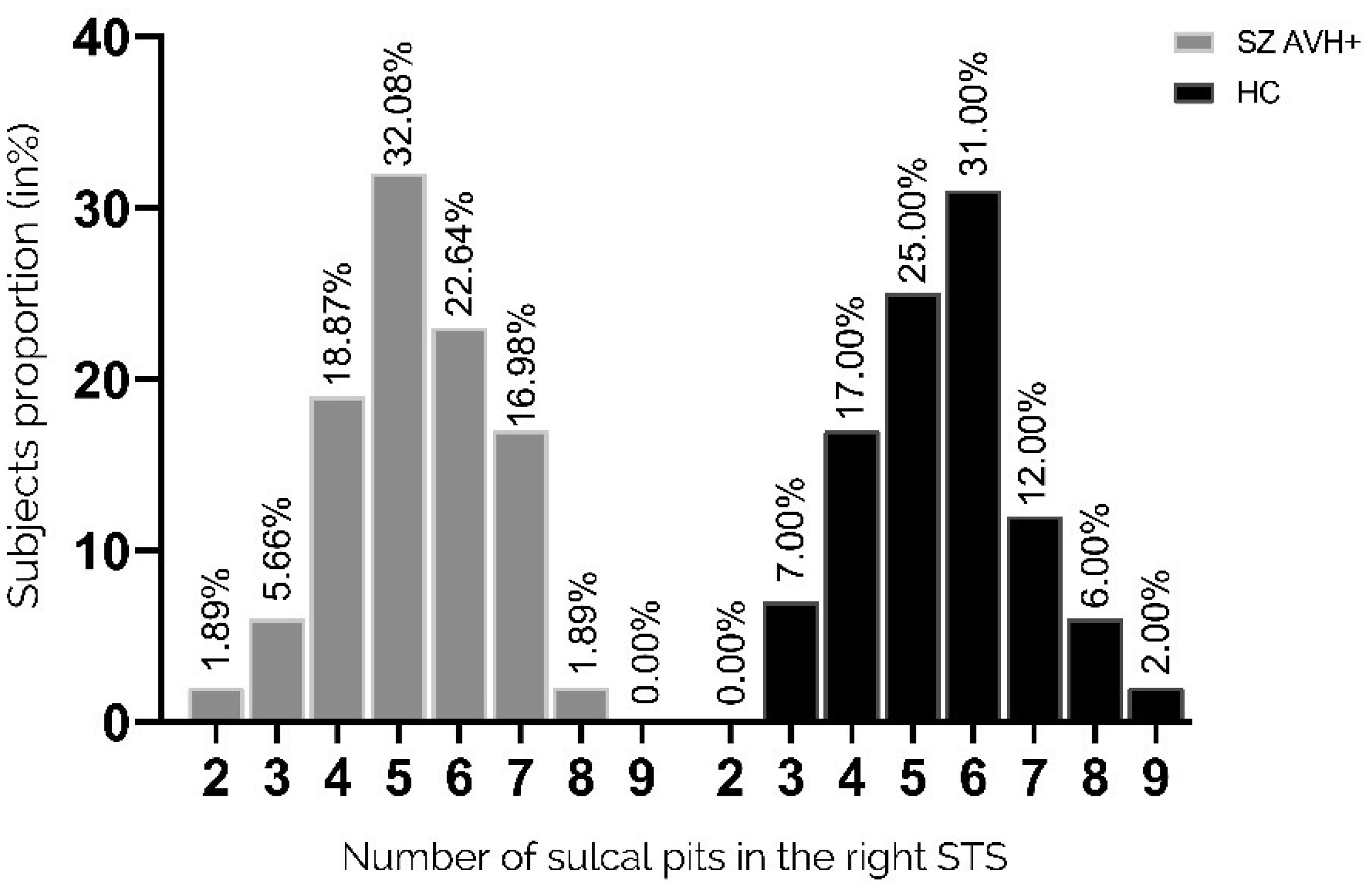
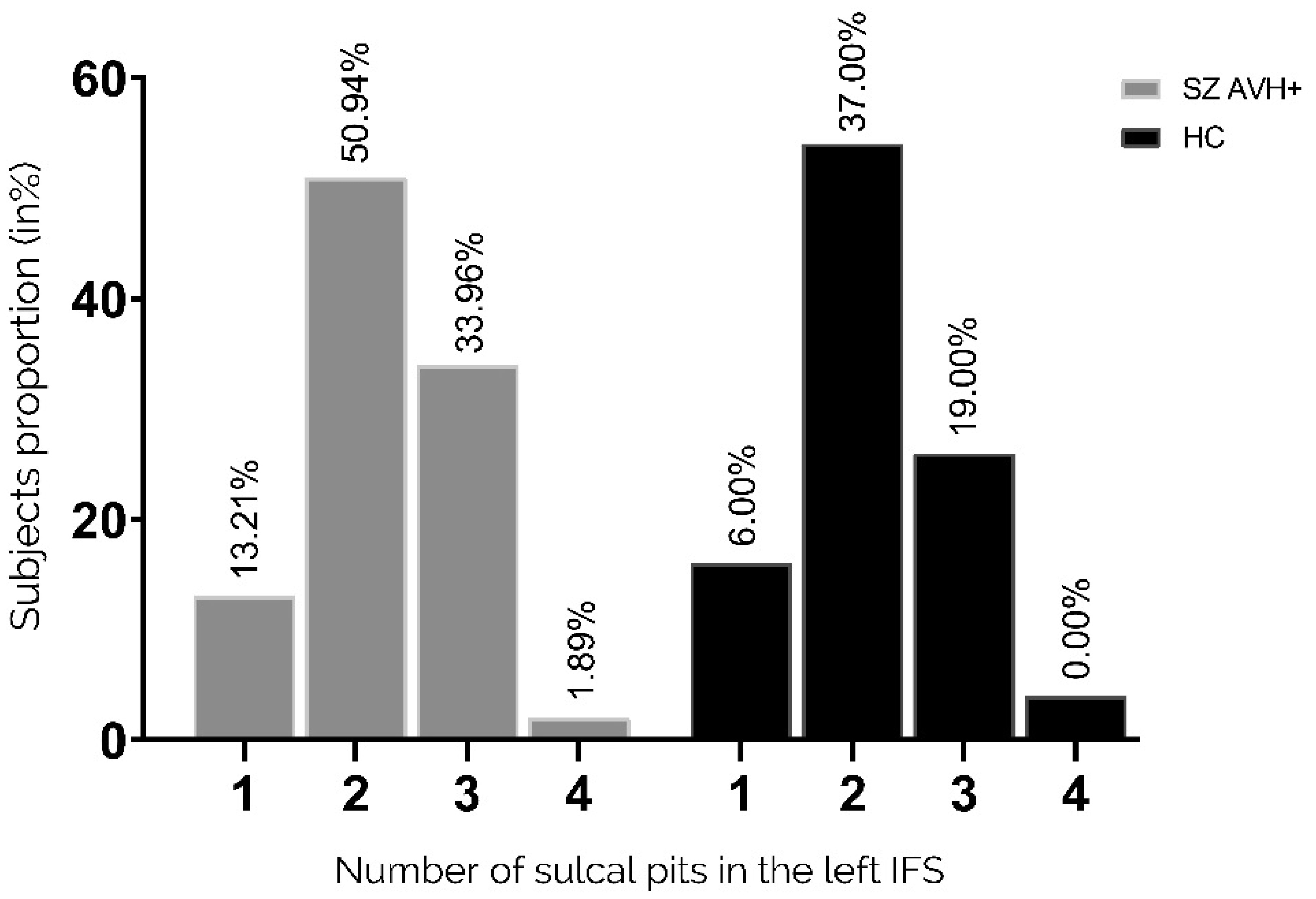
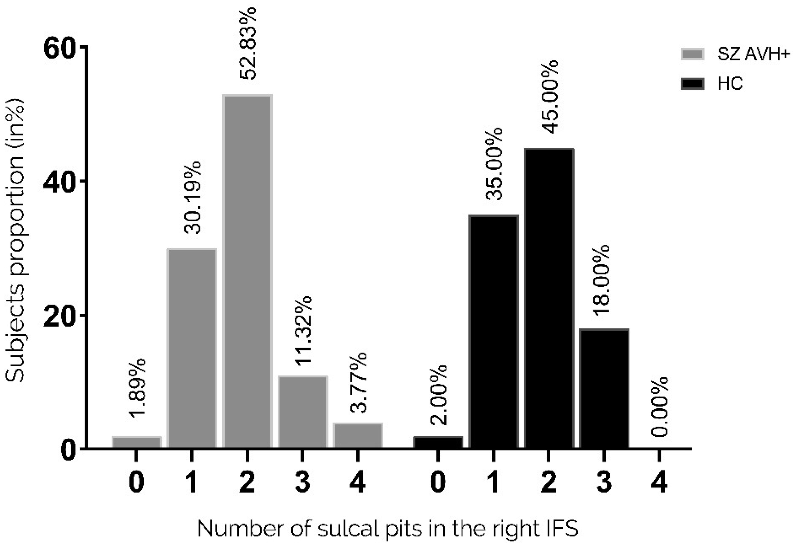
Auditory verbal hallucinations (AVHs) are among the most common and disabling symptoms of schizophrenia. They involve the superior temporal sulcus (STS), which is associated with language processing; specific STS patterns may reflect vulnerability to auditory hallucinations in schizophrenia. STS sulcal pits are the deepest points of the folds in this region and were investigated here as an anatomical landmark of AVHs. This study included 53 patients diagnosed with schizophrenia and past or present AVHs, as well as 100 healthy control volunteers. All participants underwent a 3-T magnetic resonance imaging T1 brain scan, and sulcal pit differences were compared between the two groups. Compared with controls, patients with AVHs had a significantly different distributions for the number of sulcal pits in the left STS, indicating a less complex morphological pattern. The association of STS sulcal morphology with AVH suggests an early neurodevelopmental process in the pathophysiology of schizophrenia with AVHs.
- schizophrenia,
- auditory verbal hallucination,
- structural MRI,
- superior temporal sulcus,
- sulcal pits
Citation: Baptiste Lerosier, Gregory Simon, Sylvain Takerkart, Guillaume Auzias, Sonia Dollfus. Sulcal pits of the superior temporal sulcus in schizophrenia patients with auditory verbal hallucinations[J]. AIMS Neuroscience, 2024, 11(1): 25-38. doi: 10.3934/Neuroscience.2024002

Related Papers:

Abstract

Auditory verbal hallucinations (AVHs) are among the most common and disabling symptoms of schizophrenia. They involve the superior temporal sulcus (STS), which is associated with language processing; specific STS patterns may reflect vulnerability to auditory hallucinations in schizophrenia. STS sulcal pits are the deepest points of the folds in this region and were investigated here as an anatomical landmark of AVHs. This study included 53 patients diagnosed with schizophrenia and past or present AVHs, as well as 100 healthy control volunteers. All participants underwent a 3-T magnetic resonance imaging T1 brain scan, and sulcal pit differences were compared between the two groups. Compared with controls, patients with AVHs had a significantly different distributions for the number of sulcal pits in the left STS, indicating a less complex morphological pattern. The association of STS sulcal morphology with AVH suggests an early neurodevelopmental process in the pathophysiology of schizophrenia with AVHs.

Acknowledgments

This research was conducted thanks to funding allocated to Baptiste Lerosier by the Normandy Region through its “Réseau d'Intérêt Normand” (RIN) and the French Health Ministry (PHRC, No. 06-03).

Conflicts of interest

The authors report no biomedical financial interests or potential conflicts of interest regarding this study.

References

[1]	Davis J, Eyre H, Jacka FN, et al. (2016) A review of vulnerability and risks for schizophrenia: Beyond the two-hit hypothesis. Neurosci Biobehav Rev 65: 185-194. https://doi.org/10.1016/j.neubiorev.2016.03.017
[2]	Gupta S, Kulhara P (2010) What is schizophrenia: A neurodevelopmental or neurodegenerative disorder or a combination of both? A critical analysis. Indian J Psychiatry 52: 21-27. https://doi.org/10.4103/0019-5545.58891
[3]	Pino O, Guilera G, Gómez-Benito J, et al. (2014) Neurodevelopment or neurodegeneration: review of theories of schizophrenia. Actas Esp Psiquiatr 42: 185-195.
[4]	Larøi F, Sommer IE, Blom JD, et al. (2012) The characteristic features of auditory verbal hallucinations in clinical and nonclinical groups: state-of-the-art overview and future directions. Schizophr Bull 38: 724-733. https://doi.org/10.1093/schbul/sbs061
[5]	Mueser KT, Bellack AS, Brady EU (1990) Hallucinations in schizophrenia. Acta Psychiatr Scand 82: 26-29. https://doi.org/10.1111/j.1600-0447.1990.tb01350.x
[6]	Steinmann S, Leicht G, Mulert C (2019) The interhemispheric miscommunication theory of auditory verbal hallucinations in schizophrenia. Int J Psychophysiol, The Neurophysiology of Schizophrenia: A Critical Update 145: 83-90. https://doi.org/10.1016/j.ijpsycho.2019.02.002
[7]	Gazzaniga MS (2000) Cerebral specialization and interhemispheric communication: does the corpus callosum enable the human condition?. Brain 123: 1293-1326. https://doi.org/10.1093/brain/123.7.1293
[8]	Linden DEJ, Thornton K, Kuswanto CN, et al. (2011) The brain's voices: comparing nonclinical auditory hallucinations and imagery. Cereb Cortex N. Y. N 1991 21: 330-337. https://doi.org/10.1093/cercor/bhq097
[9]	Lennox BR, Park SB, Medley I, et al. (2000) The functional anatomy of auditory hallucinations in schizophrenia. Psychiatry Res 100: 13-20. https://doi.org/10.1016/S0925-4927(00)00068-8
[10]	Shergill SS, Brammer MJ, Amaro E, et al. (2004) Temporal course of auditory hallucinations. Br J Psychiatry 185: 516-517. https://doi.org/10.1192/bjp.185.6.516
[11]	Blakemore SJ, Smith J, Steel R, et al. (2000) The perception of self-produced sensory stimuli in patients with auditory hallucinations and passivity experiences: evidence for a breakdown in self-monitoring. Psychol Med 30: 1131-1139. https://doi.org/10.1017/S0033291799002676
[12]	Modinos G, Costafreda SG, van Tol M-J, et al. (2013) Neuroanatomy of auditory verbal hallucinations in schizophrenia: a quantitative meta-analysis of voxel-based morphometry studies. Cortex 49: 1046-1055. https://doi.org/10.1016/j.cortex.2012.01.009
[13]	Köse G, Jessen K, Ebdrup BH, et al. (2018) Associations between cortical thickness and auditory verbal hallucinations in patients with schizophrenia: A systematic review. Psychiatry Res Neuroimaging 282: 31-39. https://doi.org/10.1016/j.pscychresns.2018.10.005
[14]	Mørch-Johnsen L, Nesvåg R, Jørgensen KN, et al. (2017) Auditory Cortex Characteristics in Schizophrenia: Associations With Auditory Hallucinations. Schizophr Bull 43: 75-83. https://doi.org/10.1093/schbul/sbw130
[15]	Swam C, Federspiel A, Hubl D, et al. (2012) Possible dysregulation of cortical plasticity in auditory verbal hallucinations-A cortical thickness study in schizophrenia. J Psychiatr Res 46: 1015-1023. https://doi.org/10.1016/j.jpsychires.2012.03.016
[16]	Cui Y, Liu B, Song M, et al. (2018) Auditory verbal hallucinations are related to cortical thinning in the left middle temporal gyrus of patients with schizophrenia. Psychol Med 48: 115-122. https://doi.org/10.1017/S0033291717001520
[17]	Lutterveld R, Heuvel MP, Diederen KMJ, et al. (2014) Cortical thickness in individuals with non-clinical and clinical psychotic symptoms. Brain J Neurol 137: 2664-2669. https://doi.org/10.1093/brain/awu167
[18]	Palaniyappan L, Balain V, Radua J, et al. (2012) Structural correlates of auditory hallucinations in schizophrenia: a meta-analysis. Schizophr Res 137: 169-173. https://doi.org/10.1016/j.schres.2012.01.038
[19]	Romeo Z, Spironelli C (2022) Hearing voices in the head: Two meta-analyses on structural correlates of auditory hallucinations in schizophrenia. NeuroImage: Clinical 36: 103241. https://doi.org/10.1016/j.nicl.2022.103241
[20]	Jardri R, Pouchet A, Pins D, et al. (2011) Cortical Activations During Auditory Verbal Hallucinations in Schizophrenia: A Coordinate-Based Meta-Analysis. AJP 168: 73-81. https://doi.org/10.1176/appi.ajp.2010.09101522
[21]	Chi JG, Dooling EC, Gilles FH (1977) Gyral development of the human brain. Ann Neurol 1: 86-93. https://doi.org/10.1002/ana.410010109
[22]	Dubois J, Benders M, Cachia A, et al. (2008) Mapping the early cortical folding process in the preterm newborn brain. Cereb Cortex N. Y. N 1991 18: 1444-1454. https://doi.org/10.1093/cercor/bhm180
[23]	Mangin J-F, Jouvent E, Cachia A (2010) In-vivo measurement of cortical morphology: means and meanings. Curr Opin Neurol 23: 359-367. https://doi.org/10.1097/WCO.0b013e32833a0afc
[24]	Cachia A, Borst G, Tissier C, et al. (2016) Longitudinal stability of the folding pattern of the anterior cingulate cortex during development. Dev Cogn Neurosci 19: 122-127. https://doi.org/10.1016/j.dcn.2016.02.011
[25]	Fujiwara H, Hirao K, Namiki C, et al. (2007) Anterior cingulate pathology and social cognition in schizophrenia: a study of gray matter, white matter and sulcal morphometry. NeuroImage 36: 1236-1245. https://doi.org/10.1016/j.neuroimage.2007.03.068
[26]	Garrison JR, Fernyhough C, McCarthy-Jones S, et al. (2019) Paracingulate Sulcus Morphology and Hallucinations in Clinical and Nonclinical Groups. Schizophr Bull 45: 733-741. https://doi.org/10.1093/schbul/sby157
[27]	Le Provost J-B, Bartres-Faz D, Paillere-Martinot M-L, et al. (2003) Paracingulate sulcus morphology in men with early-onset schizophrenia. Br J Psychiatry J Ment Sci 182: 228-232. https://doi.org/10.1192/bjp.182.3.228
[28]	MacKinley ML, Sabesan P, Palaniyappan L (2020) Deviant cortical sulcation related to schizophrenia and cognitive deficits in the second trimester. Transl Neurosci 11: 236-240. https://doi.org/10.1515/tnsci-2020-0111
[29]	Penttilä J, Paillére-Martinot M-L, Martinot J-L, et al. (2008) Global and temporal cortical folding in patients with early-onset schizo-phrenia. J Am Acad Child Adolesc Psychiatry 47: 1125-1132. https://doi.org/10.1097/CHI.0b013e3181825aa7
[30]	Rollins CPE, Garrison JR, Arribas M, et al. (2020) Evidence in cortical folding patterns for prenatal predispositions to hallucinations in schizophrenia. Transl Psychiatry 10: 387. https://doi.org/10.1038/s41398-020-01075-y
[31]	Cachia A, Paillère-Martinot M-L, Galinowski A, et al. (2008) Cortical folding abnormalities in schizophrenia patients with resistant auditory hallucinations. NeuroImage 39: 927-935. https://doi.org/10.1016/j.neuroimage.2007.08.049
[32]	Plaze M, Paillère-Martinot M-L, Penttilä J, et al. (2011) Where do auditory hallucinations come from?”–a brain morphometry study of schizophrenia patients with inner or outer space hallucinations. Schizophr Bull 37: 212-221. https://doi.org/10.1093/schbul/sbp081
[33]	Auzias G, Brun L, Deruelle C, et al. (2015) Deep sulcal landmarks: algorithmic and conceptual improvements in the definition and extraction of sulcal pits. NeuroImage 111: 12-25. https://doi.org/10.1016/j.neuroimage.2015.02.008
[34]	Im K, Jo HJ, Mangin J-F, et al. (2010) Spatial distribution of deep sulcal landmarks and hemispherical asymmetry on the cortical surface. Cereb Cortex N. Y. N 1991 20: 602-611. https://doi.org/10.1093/cercor/bhp127
[35]	White T, Su S, Schmidt M, et al. (2010) The development of gyrification in childhood and adolescence. Brain Cogn 72: 36-45. https://doi.org/10.1016/j.bandc.2009.10.009
[36]	Meng Y, Li G, Lin W, et al. (2014) Spatial distribution and longitudinal development of deep cortical sulcal landmarks in infants. NeuroImage 100: 206-218. https://doi.org/10.1016/j.neuroimage.2014.06.004
[37]	Yun HJ, Vasung L, Tarui T, et al. (2020) Temporal Patterns of Emergence and Spatial Distribution of Sulcal Pits During Fetal Life. Cereb Cortex N. Y. N 1991 30: 4257-4268. https://doi.org/10.1093/cercor/bhaa053
[38]	Huang Y, Zhang T, Zhang S, et al. (2023) Genetic Influence on Gyral Peaks. Neuroimage 280: 120344. https://doi.org/10.1016/j.neuroimage.2023.120344
[39]	Oldfield RC (1971) The assessment and analysis of handedness: the Edinburgh inventory. Neuropsychologia 9: 97-113. https://doi.org/10.1016/0028-3932(71)90067-4
[40]	Sheehan D, Lecrubier Y, Harnett Sheehan K, et al. (1997) The validity of the Mini International Neuropsychiatric Interview (MINI) according to the SCID-P and its reliability. Eur Psychiatry 12: 232-241. https://doi.org/10.1016/S0924-9338(97)83297-X
[41]	Dale AM, Fischl B, Sereno MI (1999) Cortical surface-based analysis. I. Segmentation and surface reconstruction. NeuroImage 9: 179-194. https://doi.org/10.1006/nimg.1998.0395
[42]	Fischl B, Sereno MI, Dale AM (1999) Cortical surface-based analysis. II: Inflation, flattening, and a surface-based coordinate system. NeuroImage 9: 195-207. https://doi.org/10.1006/nimg.1998.0396
[43]	Fischl B, Dale AM (2000) Measuring the thickness of the human cerebral cortex from magnetic resonance images. Proc Natl Acad Sci U S A 97: 11050-11055. https://doi.org/10.1073/pnas.200033797
[44]	Takerkart S, Auzias G, Brun L, et al. (2017) Structural graph-based morphometry: A multiscale searchlight framework based on sulcal pits. Med Image Anal 35: 32-45. https://doi.org/10.1016/j.media.2016.04.011
[45]	Boucher M, Whitesides S, Evans A (2009) Depth potential function for folding pattern representation, registration and analysis. Med Image Anal, Includes Special Section on Functional Imaging and Modelling of the Heart 13: 203-214. https://doi.org/10.1016/j.media.2008.09.001
[46]	Destrieux C, Fischl B, Dale A, et al. (2010) Automatic parcellation of human cortical gyri and sulci using standard anatomical nomenclature. Neuroimage 53: 1-15. https://doi.org/10.1016/j.neuroimage.2010.06.010
[47]	Palaniyappan L, Liddle PF (2012) Aberrant cortical gyrification in schizophrenia: a surface-based morphometry study. J Psychiatry Neurosci 37: 399-406. https://doi.org/10.1503/jpn.110119
[48]	Lohmann G, Cramon DY, Colchester ACF (2008) Deep sulcal landmarks provide an organizing framework for human cortical folding. Cereb Cortex N. Y. N 1991 18: 1415-1420. https://doi.org/10.1093/cercor/bhm174
[49]	Le Guen Y, Auzias G, Leroy F, et al. (2018) Genetic Influence on the Sulcal Pits: On the Origin of the First Cortical Folds. Cereb Cortex N. Y. N 1991 28: 1922-1933. https://doi.org/10.1093/cercor/bhx098
[50]	Lefrere A, Auzias G, Favre P, et al. (2023) Global and local cortical folding alterations are associated with neurodevelopmental subtype in bipolar disorders: a sulcal pits analysis. Journal of Affective Disorders 325: 224-230. https://doi.org/10.1016/j.jad.2022.12.156
[51]	Leroux E, Delcroix N, Dollfus S (2017) Abnormalities of language pathways in schizophrenia patients with and without a lifetime history of auditory verbal hallucinations: A DTI-based tractography study. World J Biol Psychiatry 18: 528-538. https://doi.org/10.1080/15622975.2016.1274053
[52]	Brun L, Auzias G, Viellard M, et al. (2016) Localized Misfolding Within Broca's Area as a Distinctive Feature of Autistic Disorder. Biol Psychiatry Cogn Neurosci Neuroimaging 1: 160-168. https://doi.org/10.1016/j.bpsc.2015.11.003

Reader Comments

Your name:*

Email:*
© 2024 the Author(s), licensee AIMS Press. This is an open access article distributed under the terms of the Creative Commons Attribution License (http://creativecommons.org/licenses/by/4.0)