Epigenetic regulation of gene expression is involved in the progression of mental disorders, including deviant behavior, brain developmental, and personality disorders. The large number of genes has been studied for their activity association with stress and depression; however, the obtained results for the majority of these genes are contradictory. The aim of our study was to investigate the possible contribution of methylation level changes to the development of personality disorders and deviant behavior. A systematic study of CpG Islands in 21 target regions, including the promoter and intron regions of the 12 genes was performed in DNA samples extracted from peripheral blood cells, to obtain an overview of their methylation status. High-throughput sequencing of converted DNA samples was performed and calling of the methylation sites on the “original top strand” in CpG islands was carried out in the Bismark pipeline. The initial methylation profile of 77 patients and 48 controls samples revealed a significant difference in 7 CpG sites in 6 genes. The most significant hypermethylation was found for the target sites of the HTR2A (p-value = 1.2 × 10⁻¹³) and OXTR (p-value = 2.3 × 10⁻⁷) genes. These data support the previous reports that alterations in DNA methylation may play an important role in the dysregulation of gene expression associated with personality disorders and deviant behavior, and confirm their potential use as biomarkers to improve thediagnosis, prognosis, and assessment of response to treatment.
Citation: I. B. Mosse, N. G. Sedlyar, K. A. Mosse, A. V. Kilchevsky. DNA methylation differences in genes associated with human personal disorders and deviant behavior[J]. AIMS Neuroscience, 2024, 11(1): 39-48. doi: 10.3934/Neuroscience.2024003
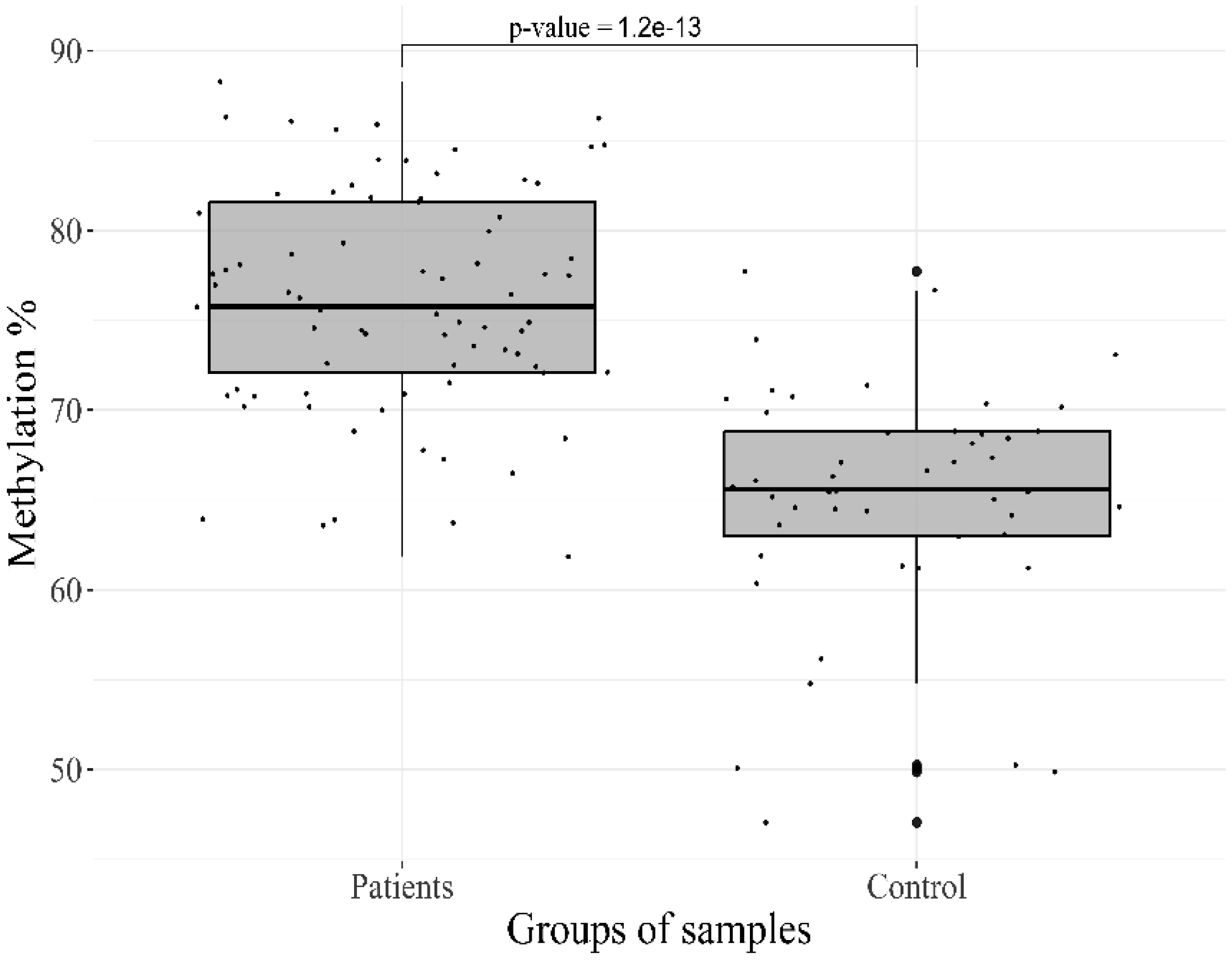
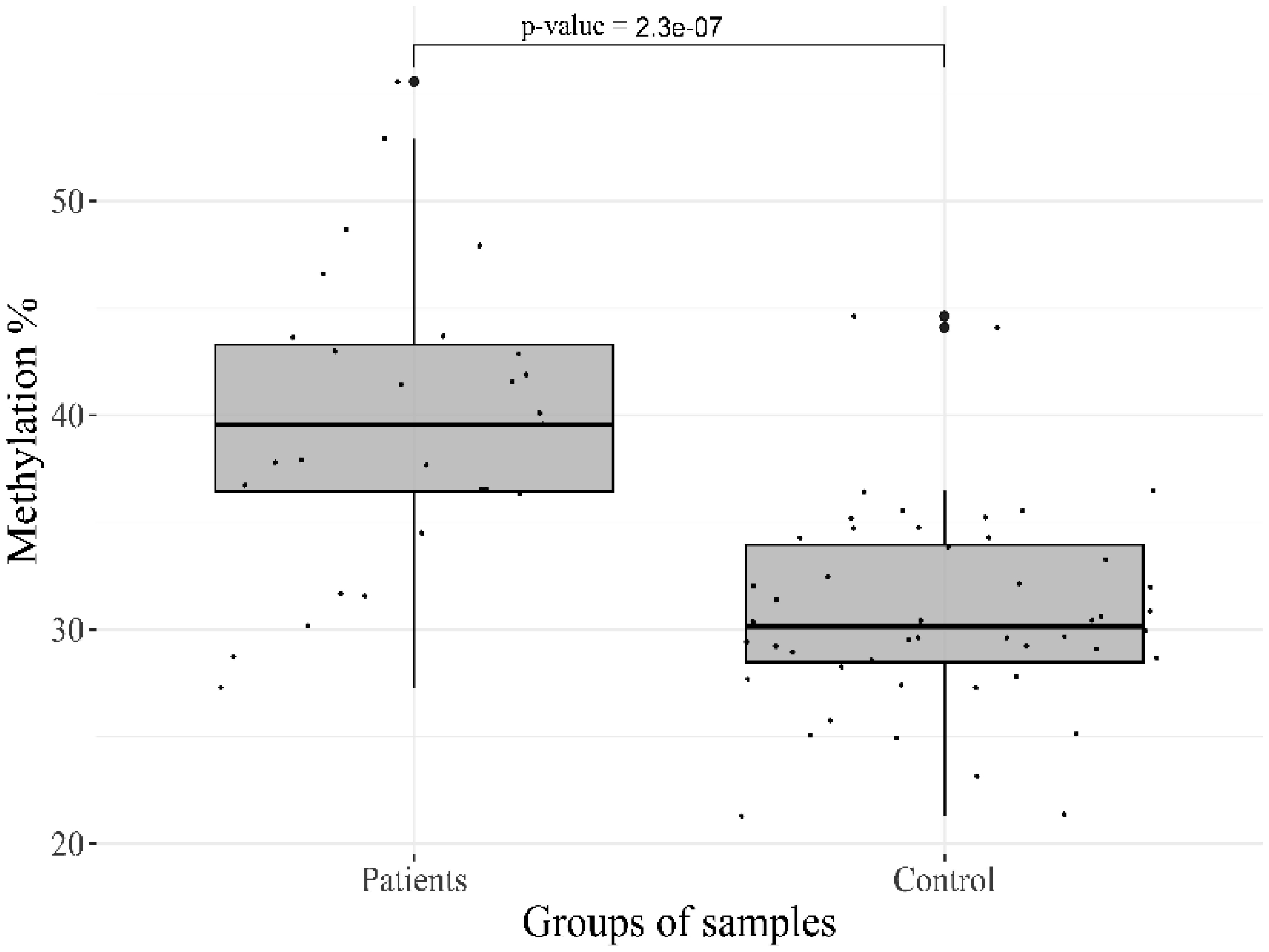
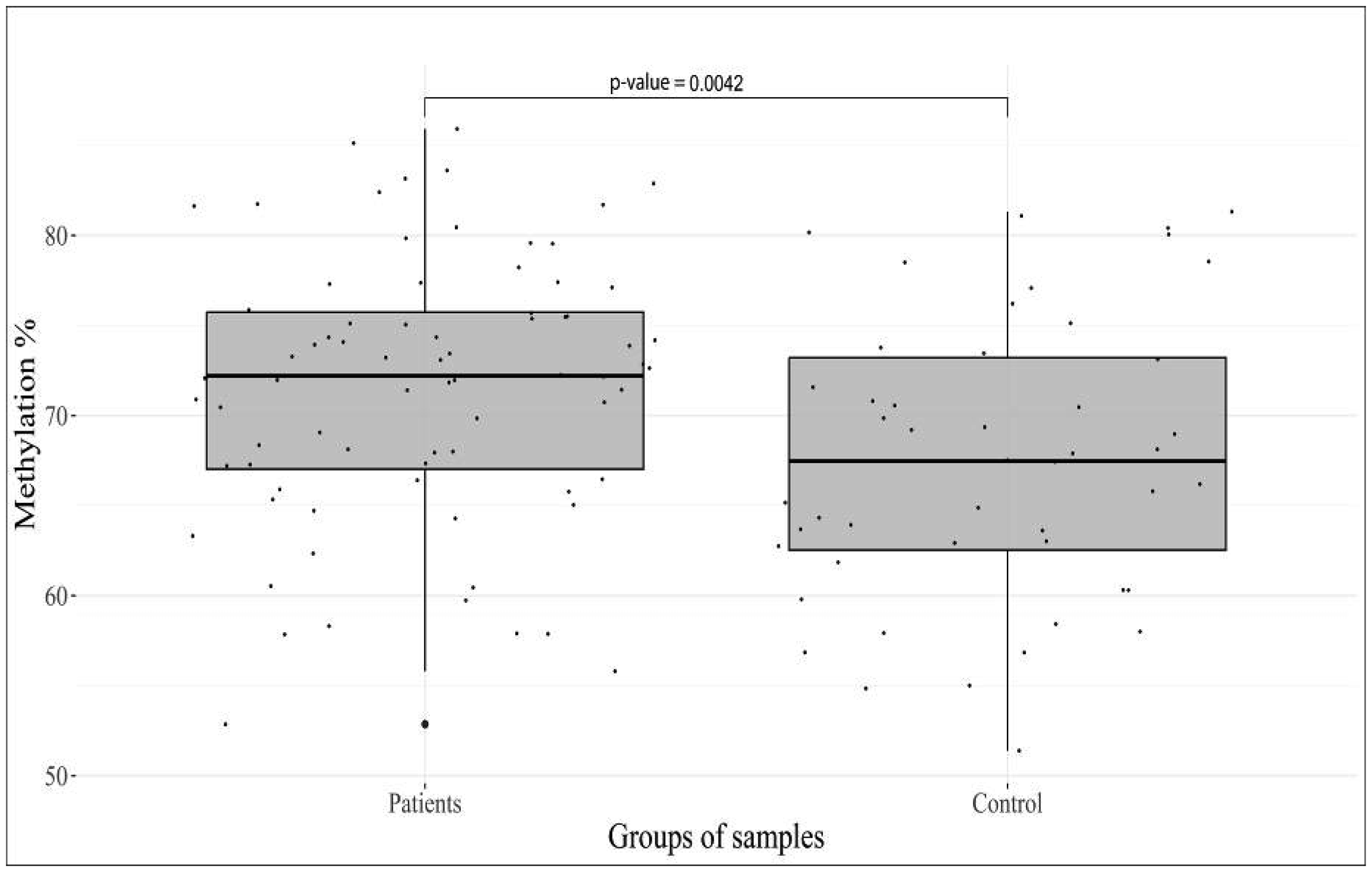
Epigenetic regulation of gene expression is involved in the progression of mental disorders, including deviant behavior, brain developmental, and personality disorders. The large number of genes has been studied for their activity association with stress and depression; however, the obtained results for the majority of these genes are contradictory. The aim of our study was to investigate the possible contribution of methylation level changes to the development of personality disorders and deviant behavior. A systematic study of CpG Islands in 21 target regions, including the promoter and intron regions of the 12 genes was performed in DNA samples extracted from peripheral blood cells, to obtain an overview of their methylation status. High-throughput sequencing of converted DNA samples was performed and calling of the methylation sites on the “original top strand” in CpG islands was carried out in the Bismark pipeline. The initial methylation profile of 77 patients and 48 controls samples revealed a significant difference in 7 CpG sites in 6 genes. The most significant hypermethylation was found for the target sites of the HTR2A (p-value = 1.2 × 10⁻¹³) and OXTR (p-value = 2.3 × 10⁻⁷) genes. These data support the previous reports that alterations in DNA methylation may play an important role in the dysregulation of gene expression associated with personality disorders and deviant behavior, and confirm their potential use as biomarkers to improve thediagnosis, prognosis, and assessment of response to treatment.

| [1] |
Bagot RC, Labonté B, Peña CJ, et al. (2014) Epigenetic signaling in psychiatric disorders: stress and depression. Dialogues Clin Neurosci 16: 281-295. https://doi.org/10.31887/DCNS.2014.16.3/rbagot 
|
| [2] |
Provencal N, Binder EB (2015) The neurobiological effects of stress as contributors to psychiatric disorders: focus on epigenetics. Curr Opin Neurobiol 30: 31-37. https://doi.org/10.1016/j.conb.2014.08.007
|
| [3] |
Rozanov VA (2012) Epigenetics: Stress and Behavior. Neurophysiology 44: 332-350. https://doi.org/10.1007/s11062-012-9304-y
|
| [4] |
Hing B, Gardner C, Potash JB (2014) Effects of negative stressors on DNA methylation in the brain: Implications for mood and anxiety disorders. Am J Med Genet B Neuropsychiatr Genet 165: 541-554. https://doi.org/10.1002/ajmg.b.32265
|
| [5] |
Keller J, Gomez R, Williams G, et al. (2017) HPA axis in major depression: cortisol, clinical symptomatology and genetic variation predict cognition. Mol Psychiatry 22: 527-536. https://doi.org/10.1038/mp.2016.120
|
| [6] |
Daut RA, Fonken LK (2019) Circadian regulation of depression: A role for serotonin. Front Neuroendocrinol 54: 100746. https://doi.org/10.1016/j.yfrne.2019.04.003
|
| [7] |
Li M, D'Arcy C, Li X, et al. (2019) What do DNA methylation studies tell us about depression? A systematic review. Transl Psychiatry 9: 1-14. https://doi.org/10.1038/s41398-019-0412-y
|
| [8] |
Goud Alladi C, Etain B, Bellivier F, et al. (2018) DNA Methylation as a Biomarker of Treatment Response Variability in Serious Mental Illnesses: A Systematic Review Focused on Bipolar Disorder, Schizophrenia, and Major Depressive Disorder. Int J Mol Sci 19: 3026. https://doi.org/10.3390/ijms19103026
|
| [9] |
Palma-Gudiel H, Córdova-Palomera A, Navarro V, et al. (2020) Twin study designs as a tool to identify new candidate genes for depression: A systematic review of DNA methylation studies. Neurosci Biobehav Rev 112: 345-352. https://doi.org/10.1016/j.neubiorev.2020.02.017
|
| [10] |
Bakusic J, Schaufeli W, Claes S, et al. (2017) Stress, burnout and depression: A systematic review on DNA methylation mechanisms. J Psychosom Res 92: 34-44. https://doi.org/10.1016/j.jpsychores.2016.11.005
|
| [11] |
Chen D, Meng L, Pei F, et al. (2017) A review of DNA methylation in depression. J Clin Neurosci 43: 39-46. https://doi.org/10.1016/j.jocn.2017.05.022
|
| [12] |
Aznar S, Klein AB (2013) Regulating prefrontal cortex activation: an emerging role for the 5-HT2A serotonin receptor in the modulation of emotion-based actions?. Mol Neurobiol 48: 841-853. https://doi.org/10.1007/s12035-013-8472-0
|
| [13] |
Ghadirivasfi M, Nohesara S, Ahmadkhaniha H-R, et al. (2011) Hypomethylation of the serotonin receptor type-2A Gene (HTR2A) at T102C polymorphic site in DNA derived from the saliva of patients with schizophrenia and bipolar disorder. Am J Med Genet Part B Neuropsychiatr Genet Off Publ Int Soc Psychiatr Genet 156B: 536-545. https://doi.org/10.1002/ajmg.b.31192
|
| [14] |
Azmitia EC (2001) Modern views on an ancient chemical: serotonin effects on cell proliferation, maturation, and apoptosis. Brain Res Bull 56: 413-424. https://doi.org/10.1016/S0361-9230(01)00614-1
|
| [15] |
Paquette AG, Lesseur C, Armstrong DA, et al. (2013) Placental HTR2A methylation is associated with infant neurobehavioral outcomes. Epigenetics 8: 796-801. https://doi.org/10.4161/epi.25358
|
| [16] |
Romano A, Tempesta B, Micioni Di Bonaventura MV, et al. (2015) From Autism to Eating Disorders and More: The Role of Oxytocin in Neuropsychiatric Disorders. Front Neurosci 9: 497. https://doi.org/10.3389/fnins.2015.00497
|
| [17] |
Quintana DS, Rokicki J, van der Meer D, et al. (2019) Oxytocin pathway gene networks in the human brain. Nat Commun 10: 668. https://doi.org/10.1038/s41467-019-08503-8
|
| [18] |
Kusui C, Kimura T, Ogita K, et al. (2001) DNA Methylation of the Human Oxytocin Receptor Gene Promoter Regulates Tissue-Specific Gene Suppression. Biochem Biophys Res Commun 289: 681-686. https://doi.org/10.1006/bbrc.2001.6024
|
| [19] |
Vaiserman AM (2012) Early-life Epigenetic Programming of Human Disease and Aging. Translational Epigenetics, Epigenetics in Human Disease . Academic Press Pages 545-567. https://doi.org/10.1016/B978-0-12-388415-2.00027-5
|
| [20] |
Danoff JS, Wroblewski KL, Graves AJ, et al. (2021) Genetic, epigenetic, and environmental factors controlling oxytocin receptor gene expression. Clin Epigenetics 13: 23. https://doi.org/10.1186/s13148-021-01017-5
|
| [21] |
Danoff JS, Connelly JJ, Morris JP, et al. (2021) An epigenetic rheostat of experience: DNA methylation of OXTR as a mechanism of early life allostasis. Compr Psychoneuroendocrinology 8: 100098. https://doi.org/10.1186/s13148-021-01017-5
|
| [22] |
Na K-S, Chang HS, Won E, et al. (2014) Association between Glucocorticoid Receptor Methylation and Hippocampal Subfields in Major Depressive Disorder. PLOS ONE 9: e85425. https://doi.org/10.1371/journal.pone.0085425
|
| [23] |
Efstathopoulos P, Andersson F, Melas PA, et al. (2018) NR3C1 hypermethylation in depressed and bullied adolescents. Transl Psychiatry 8: 1-8. https://doi.org/10.1038/s41398-018-0169-8
|
| [24] |
Knaap LJ, Oort FVA, Verhulst FC, et al. (2015) Methylation of NR3C1 and SLC6A4 and internalizing problems. The TRAILS study. J Affect Disord 180: 97-103. https://doi.org/10.1016/j.jad.2015.03.056
|
| [25] |
Weaver IC (2007) Epigenetic programming by maternal behavior and pharmacological intervention. Nature versus nurture: Let's call the whole thing off. Epigenetics 2: 22-28. https://doi.org/10.4161/epi.2.1.3881
|
| [26] |
Zannas AS, Wiechmann T, Gassen NC, et al. (2016) Gene-stress-epigenetic regulation of FKBP5: Clinical and translational implications. Neuropsychopharmacology 41: 261-274. https://doi.org/10.1038/npp.2015.235
|
| [27] |
Thomassin H, Flavin M, Espinas ML, et al. (2001) Glucocorticoid-induced DNA demethylation and gene memory during development. EMBO J 20: 1974-1983. https://doi.org/10.1093/emboj/20.8.1974
|
Figures(3) / Tables(2)

I. B. Mosse, N. G. Sedlyar, K. A. Mosse, A. V. Kilchevsky. DNA methylation differences in genes associated with human personal disorders and deviant behavior[J]. AIMS Neuroscience, 2024, 11(1): 39-48. doi: 10.3934/Neuroscience.2024003


 DownLoad: