Gut neurotoxin p-cresol induces brain-derived neurotrophic factor secretion and increases the expression of neurofilament subunits in PC-12 cells

Gigi Tevzadze; Tamar Barbakadze; Elisabed Kvergelidze; Elene Zhuravliova; Lali Shanshiashvili; David Mikeladze; Gigi Tevzadze; Tamar Barbakadze; Elisabed Kvergelidze; Elene Zhuravliova; Lali Shanshiashvili; David Mikeladze

doi:10.3934/Neuroscience.2022002

AIMS Neuroscience

2022, Volume 9, Issue 1: 12-23. doi: 10.3934/Neuroscience.2022002

Previous Article Next Article

Research article

Gut neurotoxin p-cresol induces brain-derived neurotrophic factor secretion and increases the expression of neurofilament subunits in PC-12 cells

1.
4-D Research Institute, Ilia State University, 3/5 Cholokashvili av, Tbilisi, 0162, Georgia
2.
School of Natural Sciences and Medicine, Institute of Chemical Biology, Ilia State University, 3/5 Cholokashvili ave, Tbilisi, 0162, Georgia
3.
I. Beritashvili Center of Experimental Biomedicine 14, Gotua Str., Tbilisi 0160, Georgia

Received: 01 October 2021 Revised: 30 November 2021 Accepted: 19 December 2021 Published: 23 December 2021

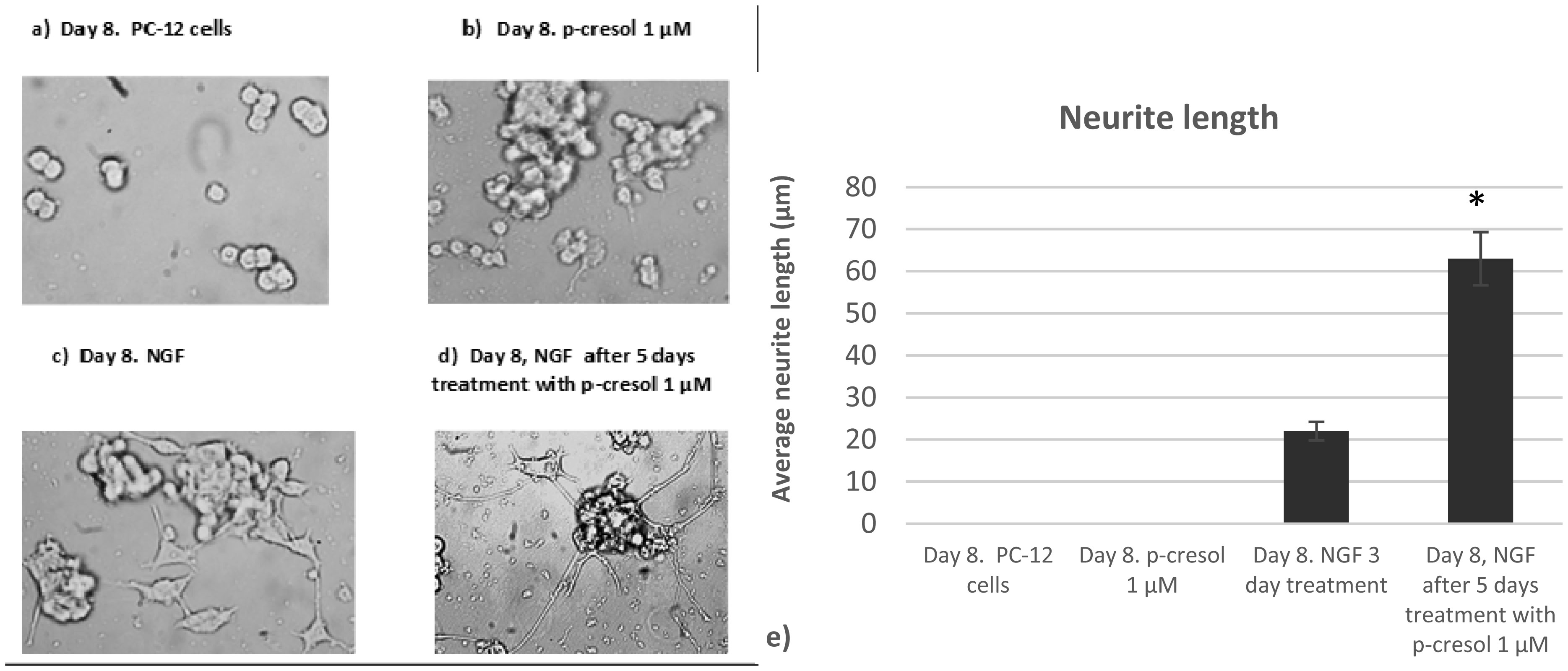
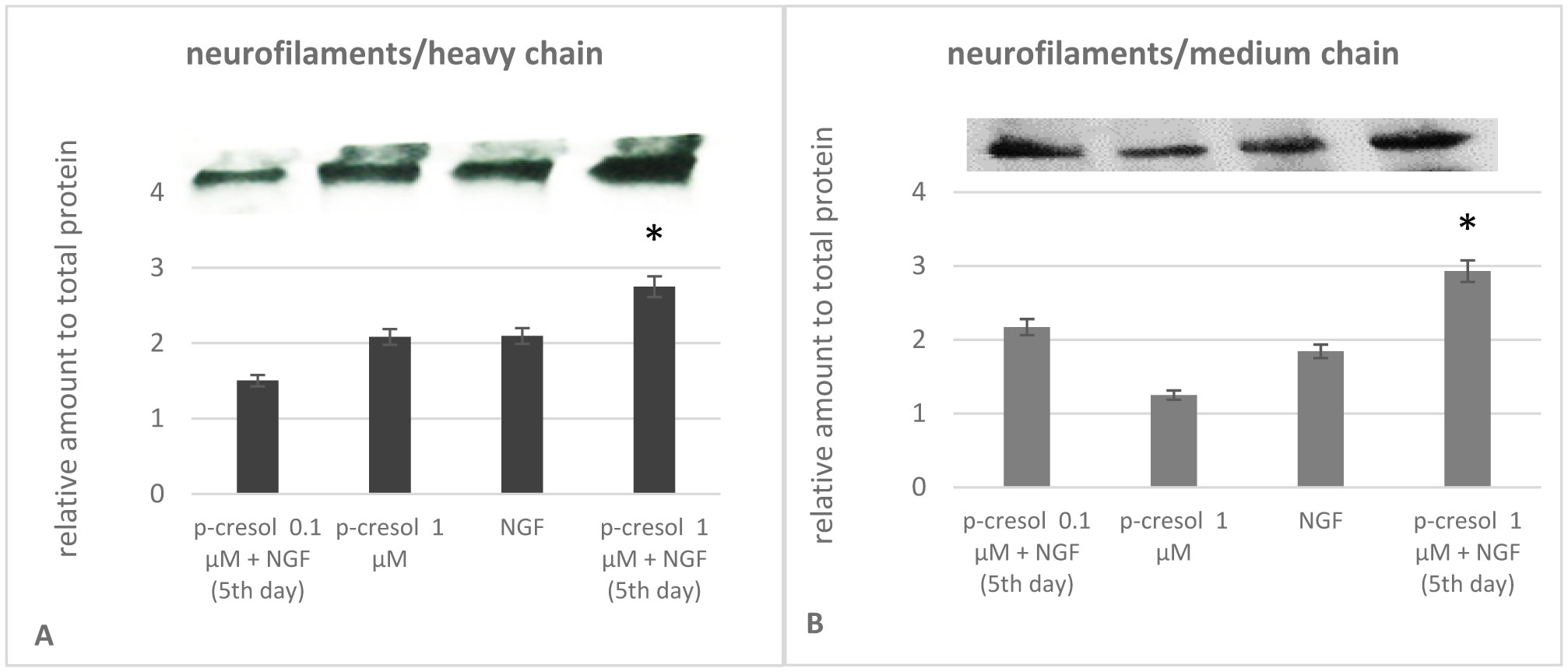
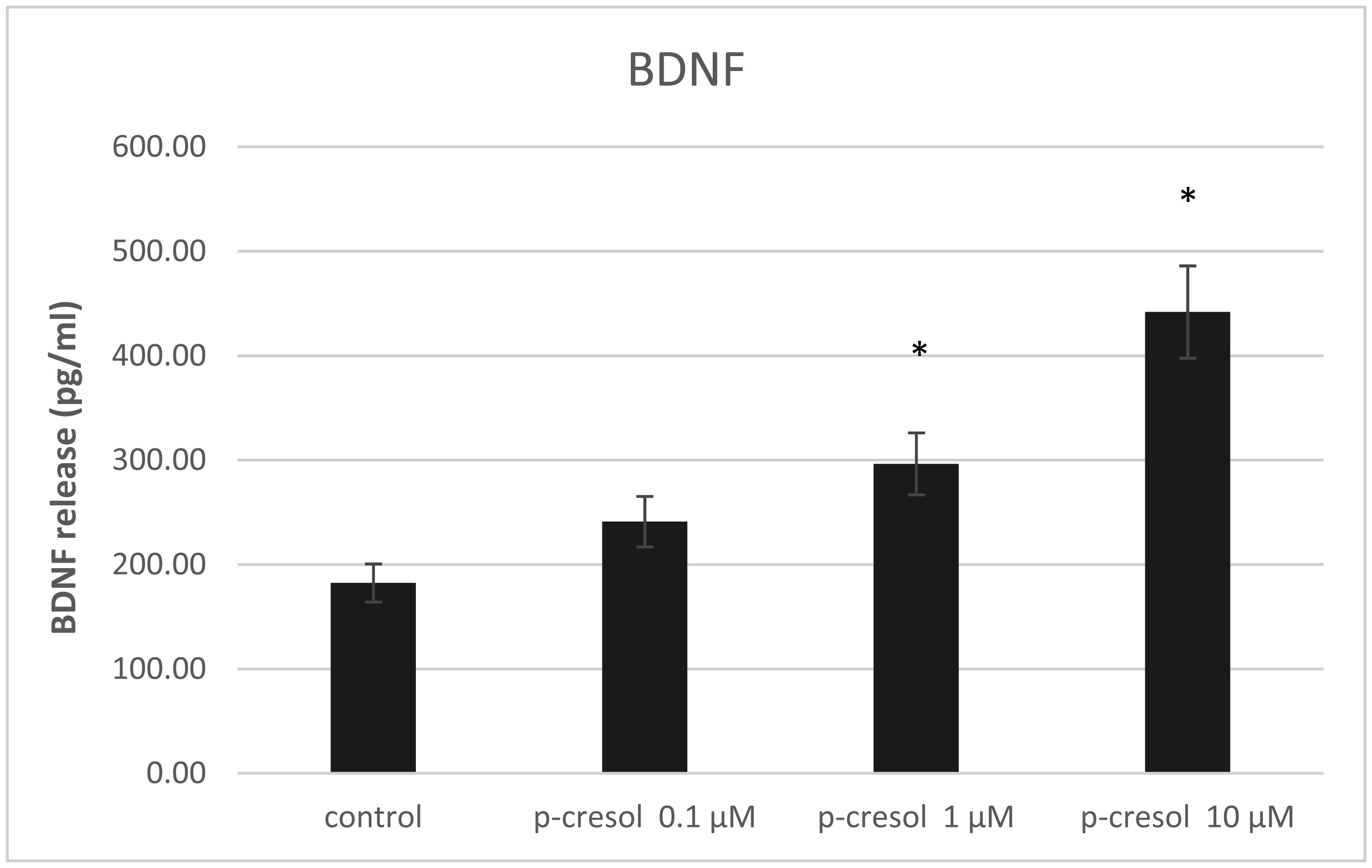
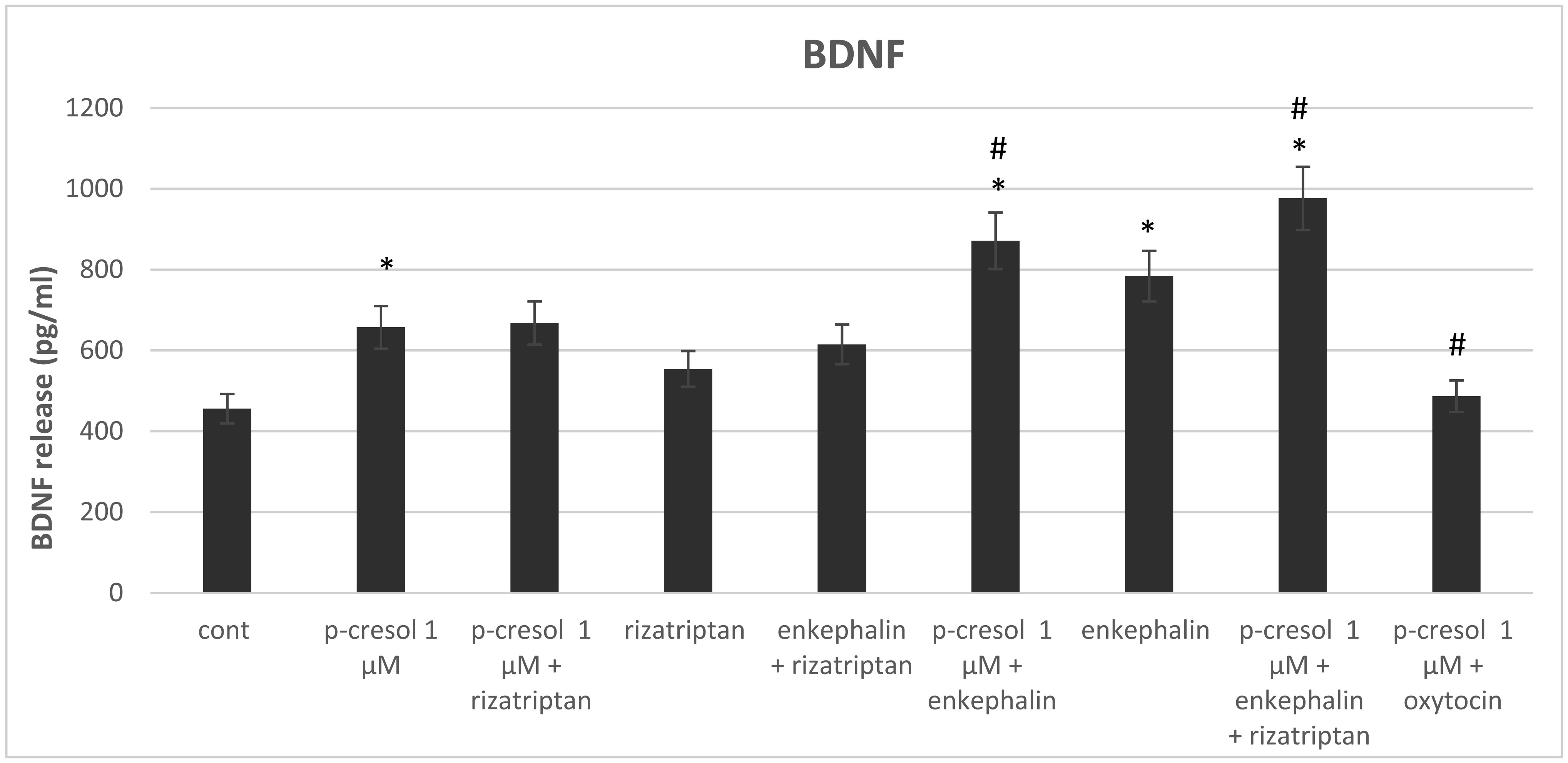
Increased p-cresol levels reportedly alter brain dopamine metabolism and exacerbate neurological disorders in experimental animals. In contrast to toxic concentrations, low doses of p-cresol may have distinct effects on neuronal metabolism. However, the role of p-cresol in synapse remodeling, neurite outgrowth, and other anabolic processes in neurons remains elusive. We propose that low doses of p-cresol affect neuronal cell structural remodeling compared with the high concentration-mediated harmful effects. Thus, the effects of p-cresol on the secretion of brain-derived neurotrophic factor (BDNF) and neurofilament subunit expression were examined using rat pheochromocytoma cells (PC-12 cells). We observed that low doses of p-cresol potentiated nerve growth factor-induced differentiation via secretion of BDNF in cultured PC-12 cells. Opioidergic compounds modulated these p-cresol effects, which were reversed by oxytocin. We propose that this effect of p-cresol has an adaptive and compensatory character and can be attributed to the induction of oxidative stress. Accordingly, we hypothesize that low doses of p-cresol induce mild oxidative stress, stimulating BDNF release by activating redox-sensitive genes. Given that the intestinal microbiome is the primary source of endogenous p-cresol, the balance between gut microbiome strains (especially Clostridium species) and opioidergic compounds may directly influence neuroplasticity.

Keywords:

Citation: Gigi Tevzadze, Tamar Barbakadze, Elisabed Kvergelidze, Elene Zhuravliova, Lali Shanshiashvili, David Mikeladze. Gut neurotoxin p-cresol induces brain-derived neurotrophic factor secretion and increases the expression of neurofilament subunits in PC-12 cells[J]. AIMS Neuroscience, 2022, 9(1): 12-23. doi: 10.3934/Neuroscience.2022002

Related Papers:

[1]	Hongyan Dui, Yong Yang, Xiao Wang . Reliability analysis and recovery measure of an urban water network. Electronic Research Archive, 2023, 31(11): 6725-6745. doi: 10.3934/era.2023339
[2]	Xu Zhan, Yang Yong, Wang Xiao . Phased mission reliability analysis of unmanned ship systems. Electronic Research Archive, 2023, 31(10): 6425-6444. doi: 10.3934/era.2023325
[3]	Majed Alowaidi, Sunil Kumar Sharma, Abdullah AlEnizi, Shivam Bhardwaj . Integrating artificial intelligence in cyber security for cyber-physical systems. Electronic Research Archive, 2023, 31(4): 1876-1896. doi: 10.3934/era.2023097
[4]	Xiaoyang Xie, Shanghua Wen, Minglong Li, Yong Yang, Songru Zhang, Zhiwei Chen, Xiaoke Zhang, Hongyan Dui . Resilience evaluation and optimization for an air-ground cooperative network. Electronic Research Archive, 2024, 32(5): 3316-3333. doi: 10.3934/era.2024153
[5]	Shuang Yao, Dawei Zhang . A blockchain-based privacy-preserving transaction scheme with public verification and reliable audit. Electronic Research Archive, 2023, 31(2): 729-753. doi: 10.3934/era.2023036
[6]	Shanpu Gao, Yubo Li, Anping Wu, Hao Jiang, Feng Liu, Xinlong Feng . An intelligent optimization method for accelerating physical quantity reconstruction in computational fluid dynamics. Electronic Research Archive, 2025, 33(5): 2881-2924. doi: 10.3934/era.2025127
[7]	Wanxun Jia, Ling Li, Haoyan Zhang, Gengxiang Wang, Yang Liu . A novel nonlinear viscous contact model with a Newtonian fluid-filled dashpot applied for impact behavior in particle systems. Electronic Research Archive, 2025, 33(5): 3135-3157. doi: 10.3934/era.2025137
[8]	Sida Lin, Jinlong Yuan, Zichao Liu, Tao Zhou, An Li, Chuanye Gu, Kuikui Gao, Jun Xie . Distributionally robust parameter estimation for nonlinear fed-batch switched time-delay system with moment constraints of uncertain measured output data. Electronic Research Archive, 2024, 32(10): 5889-5913. doi: 10.3934/era.2024272
[9]	Yunying Huang, Wenlin Gui, Yixin Jiang, Fengyi Zhu . Types of systemic risk and macroeconomic forecast: Evidence from China. Electronic Research Archive, 2022, 30(12): 4469-4492. doi: 10.3934/era.2022227
[10]	Yazhou Chen, Dehua Wang, Rongfang Zhang . On mathematical analysis of complex fluids in active hydrodynamics. Electronic Research Archive, 2021, 29(6): 3817-3832. doi: 10.3934/era.2021063

Abstract

1. Introduction

Let $q$ be a power of odd prime. Several researchers have looked into a variety of properties about the primitive roots modulo $q$ . Let $g_1, g_2$ represent two primitive roots modulo $q$ , $a$ , $b$ and $c$ represent arbitrary non-zero elements in $\mathbb{F}_q$ . Is there some $q_0$ such that for all $q > q_0$ , there is always one representation

$\begin{eqnarray} a = bg_1+cg_2\ ? \end{eqnarray}$

(1.1)

For $b = 1$ and $c = -1$ , Vegh ^[1] considered a specific form of Eq (1.1), which is known as Vegh's Conjecture, (see [,§ F9] for further details). Cohen ^[3] demonstrated Vegh's Conjecture for all $q > 7$ .

For $b = 1$ and $c = 1$ , Golomb ^[4] proposed another specific form of Eq (1.1). This was proved by Sun ^[5] for $q > 2^{60}\approx 1.15\times 10^{18}$ .

Moreover, Cohen et al. ^[6] studied linear sums of primitive roots and their inverses in finite fields $\mathbb{F}_q$ and showed that if $q > 13$ , then for arbitrary non-zero $a, b \in \mathbb{F}_q$ , there is a pair of primitive elements ( $g_1$ , $g_2$ ) of $\mathbb{F}_q$ such that both $ag_1+bg_2$ and $ag^{-1}_1+bg^{-1}_2$ are primitive.

Let $p$ be an odd prime. Carlitz ^[7] relied on some results of Davenport and obtained for any $k-1$ fixed integers $c_1, c_2, \ldots, c_{k-1}$ with $c_i \geq 1 (i = 1, 2, \ldots, k-1)$ . Let $g, g_1, \ldots, g_{k-1}$ be primitive roots modulo $p$ and $N_k$ denote the number of $g\bmod p$ such that $g_1-g = c_1, \ldots, g_{k-1}-g = c_{k-1}$ . Then

$\begin{eqnarray*} N_k \sim \frac{\phi^{k}(p-1)}{p^{k-1}}\ \hfill (p\rightarrow \infty). \end{eqnarray*}$

More results of the primitive roots distribution can be found in ^[8,9,10,11].

Lehmer [,§ F12] proposed the definition of $Lehmer~~ number$ , according to which $a$ is a $Lehmer ~~number$ if and only if $a$ and $\bar{a}$ have opposite parity, i.e., $(2, a+\bar{a}) = 1$ , where $\bar{a}$ is the multiplicative inverse of $a$ modulo $p$ . It is simple to demonstrate that there are no Lehmer numbers modulo $p$ when $p = 3$ or $7$ . Zhang ^[12] established that if $M_p$ denotes the number of Lehmer numbers modulo $p$ , then

$\begin{eqnarray*} M_p = \frac{p-1}{2}+\mathrm{O}\left(p^{\frac{1}{2}}\ln^2p\right). \end{eqnarray*}$

A Lehmer number that is also a primitive root modulo $p$ will be called a $Lehmer~~ primitive~~ root$ or an $LPR$ . The inverse of an $LPR$ is also an $LPR$ . We assume that $p > 3$ because there is no Lehmer number modulo $3$ . Wang and Wang ^[13] investigated the distribution of $LPRs$ involving Golomb's conjecture. Let $G_p$ denote the number of Golomb pairs $(a, b)$ (i.e., $a+b\equiv 1(\bmod\; p)$ ) are $LPRs$ . They showed

$\begin{eqnarray*} G_p = \frac{1}{4}\frac{\phi^2(p-1)}{p-1}+O\left(\frac{\phi^2(p-1)}{p^{\frac{5}{4}}}\cdot 4^{\omega(p-1)}\cdot \ln^2p\right). \end{eqnarray*}$

Let $N_p$ denote the number of $LPRs$ modulo $p$ . For odd integers $m\geq 3$ , define the positive number $T_m$ by

$\begin{eqnarray*} T_m = \frac{2}{m\ln m}\sum\limits_{j = 1}^{(m-1)/2}\tan\left(\frac{\pi j}{m}\right). \end{eqnarray*}$

Cohen and Trudgian ^[14] improved the result of Wang and Wang ^[13] and showed

$\begin{eqnarray*} \left|N_p-\frac{\phi(p-1)}{2}\right| < T_p^2\frac{\phi(p-1)}{p-1}2^{\omega(p-1)}p^{\frac{1}{2}}\ln^2p \end{eqnarray*}$

and

$\begin{eqnarray*} \left|G_p-\frac{\phi^2(p-1)}{4(p-1)^2}(p-2)\right| < \frac{\phi^2(p-1)}{4(p-1)^2}T_p^2[2^{2\omega(p-1)}(9\ln^2p+1)-1]p^{\frac{1}{2}}, \end{eqnarray*}$

where $\frac{2}{\pi}\left(1+\frac{0.548}{\ln p}\right) < T_p < \frac{2}{\pi}\left(1+\frac{1.549}{\ln p}\right)$ .

Specifically, they obtained that for an odd prime $p(\neq 3, 7)$ , there exists an $LPR$ modulo $p$ .

Inspired by the results of Cohen and Trudgian ^[14] and Wang and Wang ^[13], we mainly studied the distribution of $LPRs$ modulo $p$ related to the Golomb's conjecture in two aspects. On the one hand, we extend Eq (1.1) to the case involving $k > 1$ variables. Let $\mathcal{R}$ be set of $LPRs$ modulo $p$ that is a subset of ${\mathbb{F}}_p$ . $a_1, a_2, \ldots, a_k, c$ are non-zero elements in ${\mathbb{F}}_p$ and $N(\mathcal{R}, p)$ denotes the number of solutions of the equation

$\begin{eqnarray*} a_1g_1+a_2g_2+\cdots+a_kg_k = c, \ g_1, g_2, \ldots, g_k \in \mathcal{R}. \end{eqnarray*}$

We consider the distribution properties of $N(\mathcal{R}, p)$ , and obtain the following:

Theorem 1. Let $p > 3$ be an odd prime. Then we have

$\begin{eqnarray*} N(\mathcal{R}, p) = \frac{\phi^k(p-1)}{2^kp}+\mathrm{O}\left(\frac{\phi^k(p-1)}{p^\frac{3}{2}}2^{k\omega(p-1)}\ln^{2k}p\right), \end{eqnarray*}$

where the symbol $\mathrm{O}$ is dependent on $k$ .

When $k = 2$ , we can obtain the number of the Golomb pairs that are $LPRs$ .

On the other hand, we consider the distribution of $k$ consecutive $LPRs$ and generalize it to a more general form.

Let $f(x)\in \mathbb{F}_p[x]$ . Define

$\begin{eqnarray*} M(f(x), \mathcal{R}, p) = \#\{x: 1\leq x\leq p-1, f(x+c_1), f(x+c_2), \cdots, f(x+c_k) \in \mathcal{R} \}. \end{eqnarray*}$

Then we have:

Theorem 2. Let $f(x)\in \mathbb{F}_p[x]$ with degree $l\geq 1$ . $c_1, c_2, \ldots, c_k$ are distinct elements in $\mathbb{F}_p$ . Suppose that one of the following conditions holds:

$\rm (i)$ $f(x)$ is irreducible,

$\rm (ii)$ $f(x)$ has no multiple zero in $\bar{\mathbb{F}}_p$ and $k = 2$ ,

$\rm (iii)$ $f(x)$ has no multiple zero in $\bar{\mathbb{F}}_p$ and $(4k)^{l} < p$ .

Then we have

$\begin{eqnarray*} &&M(f(x), \mathcal{R}, p) = \frac{1}{2^k}\frac{\phi^k(p-1)}{(p-1)^{k-1}}+\mathrm{O}\left(\frac{\phi^k(p-1)}{p^{k-\frac{1}{2}}}2^{k\omega(p-1)}\ln^{2k}p\right), \end{eqnarray*}$

where the symbol $\mathrm{O}$ is dependent on $k$ and $l$ .

Take $f(x) = x$ , $c_k = 0$ in Theorem 2. Then we can get the number of $k$ consecutive primitive roots $x, x+c_1, \ldots, x+c_{k-1}$ are Lehmer numbers, which is:

Corollary 1. Let $p$ be an odd prime. Then for any $1\leq\ x\leq(p-1)$ that is an LPR modulo $p$ , we have

$\begin{eqnarray*} &&M(x, \mathcal{R}, p) = \frac{1}{2^k}\frac{\phi^k(p-1)}{(p-1)^{k-1}}+\mathrm{O}\left(\frac{\phi^k(p-1)}{p^{k-\frac{1}{2}}}2^{k\omega(p-1)}\ln^{2k}p\right), \end{eqnarray*}$

where the symbol $\mathrm{O}$ is dependent on $k$ .

When $k = 1, 2$ , we can easily deduce the Theorem 1 and Theorem 6 in Cohen and Trudgian ^[14], respectively.

Notation: Throughout this paper, $\mathbb{F}_q$ denotes a finite field of characteristic $p$ , $\bar{\mathbb{F}}_q$ denotes the algebraic closure of $\mathbb{F}_q$ , $\phi(n)$ is reserved for the Euler function, $\mu(n)$ is the M $\ddot{o}$ bius function. We use $\omega(n)$ to denote the number of all distinct prime divisors of $n$ . Write $\sum_{\chi_d}$ to denote a sum over all $\phi(d)$ multiplicative characters $\chi_d$ of order $d$ over ${\mathbb{F}}_p$ , and denote by $\mathop{\sum_{n = 1}^{p}}^{'}$ the summation of $1\leq n\leq p$ with $(n, p) = 1$ . $\tau(\chi)$ is the classical Gauss sums associated with character $\chi$ mudulo $p$ . $f\ll g$ means $|f|\leq cg$ with some positive constant $c$ , $f = \mathrm{O}(g)$ means $f\ll g$ .

2. Some lemmas

To complete the proof of the theorems, we need following several lemmas. The proofs of these lemmas require some basic knowledge of analytic number theory, which can be found in ^[15].

Lemma 1. Let $p$ be an odd prime. Then for any integer $a$ coprime to $p$ (i.e., $(a, p) = 1$ ), we have the identity

$\frac{\phi(p-1)}{p-1}\sum\limits_{d\mid p-1}\frac{\mu(d)}{\phi(d)}\sum\limits_{\chi_d}\chi_d(a) = \left\{ \begin{array}{ll} 1, &\ { if~~ a ~~ is ~~ a~~ primitive ~~ root ~~ \text{mod}~~ p;}\\ 0, &\ {if~~ a ~~ is~~ not~~ a~~ primitive~~ root~~ \text{mod}~~ p.} \end{array}\right.$

Proof. See Proposition 2.2 of Narkiewicz ^[16]. □

Lemma 2. Let $p$ be an odd prime, $\chi$ be a nonprincipal multiplicative character modulo $p$ of order $d$ . Suppose $g(x)\in \mathbb{F}_p[x]$ has precisely $m$ distinct ones among its zeros, and suppose that $g(x)$ is not the constant multiple of a $d$ -th power over $\mathbb{F}_q$ . Then

$\left|\sum\limits_{x\in \mathbb{F}_p}\chi\left(g(x)\right)\right|\leq \left(m-1\right)\cdot p^{\frac{1}{2}}.$

Proof. See Theorem 2C in Chapter 2 of Schmidt ^[17]. □

Lemma 3. Let $\mathbb{F}_q$ be a finite field of characteristic $p$ , $\psi$ be a nontrivial additive character and $\chi$ be a nonprincipal multiplicative character on $\mathbb{F}_q$ of order $d$ . For two rational functions $f(x), g(x)\in\mathbb{F}_q[x]$ , define $K(\psi, f;\chi, g) = \sum_{x\in\mathbb{F}_q\backslash S}\chi(g(x))\psi(f(x))$ , where $S$ denotes the set of poles of $f(x)$ and $g(x)$ . Suppose the following conditions hold:

$\rm (i)$ $g(x)$ is not the constant multiple of a $d$ -th power over $\mathbb{F}_q$ .

$\rm (ii)$ $f(x)$ is not of the form $(h(x))^p-h(x)$ with a rational function $h(x)$ over $\mathbb{F}_q$ .

Then we have

$|K(\psi, f;\chi, g)|\leq(\deg(f)+m-1)\sqrt{q},$

where $m$ is the number of distinct roots and (noninfinite) poles of $g(x)$ in $\mathbb{F}_q$ .

Proof. See Theorem 2G in Chapter 2 of Schmidt ^[17]. □

Lemma 4. Let $p$ be an odd prime. Let $c_1, \cdots, c_k$ be distinct elements in $\mathbb{F}_p$ . Assume that $f(x)\in\mathbb{F}_{p}[x]$ with $\deg(f) = l$ . Define the polynomial

$h(x) = f(x+c_1)\cdots f(x+c_k).$

Suppose one of the following conditions holds:

$\rm (i)$ $f(x)$ is irreducible,

$\rm (ii)$ $f(x)$ has no multiple zero in $\bar{\mathbb{F}}_p$ and $k = 2$ ,

$\rm (iii)$ $f(x)$ has no multiple zero in $\bar{\mathbb{F}}_p$ and $(4k)^{l} < p$ .

Then $h(x)$ has at least one simple root in $\bar{\mathbb{F}}_p$ .

Proof. Suppose that $f(x)$ is irreducible. Then $f(x+c_1), \cdots, f(x+c_k)$ are distinct irreducible polynomials, and $h(x)$ has at least $k$ simple roots in $\bar{\mathbb{F}}_p$ . The cases of $\rm (ii)$ and $\rm (iii)$ can be proved by Theorem 2 and Lemma 2 of ^[18], for $k = 2$ or $(4k)^{l} < p$ , $(l, k, p)$ is "admissible triple, " then $f(x+c_1)\cdots f(x+c_k)$ has at least one simple root. □

Lemma 5. Let $p$ be an odd prime, $m_1, \ldots, m_k, n_1, \ldots, n_k$ be integers with $(m_1\cdots m_kn_1\cdots n_k, p) = 1$ , and polynomials $g(x), f_1(x), \ldots, f_k(x)\in\mathbb{F}_p[x]$ . Let $\chi$ be a Dirichlet character modulo $p$ of order $d$ . Define

$\begin{eqnarray*} &&K(\chi, g, f_1, \cdots, f_k;p)\\ && = \mathop{\sum\limits_{x = 1}^{p}}_{(f_1(x)\cdots f_k(x), p) = 1}\chi(g(x)) e\left(\frac{m_1f_1(x)+\cdots+m_kf_k(x)+n_1\overline{f_1(x)}+\cdots+n_k\overline{f_k(x)}}{p}\right). \end{eqnarray*}$

Suppose the following conditions hold:

$\rm (i)$ $g(x)$ can not be the constant multiple of a $d$ -th power over $\mathbb{F}_p$ .

$\rm (ii)$ $F(x) = f_1(x)\cdots f_k(x)$ has at least one simple root in $\bar{\mathbb{F}}_p$ .

Then we have

$\begin{eqnarray*} |K(\chi, g, f_1, \cdots, f_k;p)| \leq\left(\max(\deg(f_1), \cdots, \deg(f_k))+l\right)\sqrt{p}, \end{eqnarray*}$

where $e(x) = e^{2\pi ix}$ and $l$ is the number of distinct roots of $g(x)$ in $\bar{\mathbb{F}}_p$ .

Proof. It is clear that

$\begin{eqnarray*} &&m_1f_1(x)+\cdots+m_kf_k(x)+n_1\overline{f_1(x)}+\cdots+n_k\overline{f_k(x)}\\ && = \frac{F(x)(m_1f_1(x)+\cdots+m_kf_k(x))+n_1\frac{F(x)}{f_1(x)}+\cdots +n_k\frac{F(x)}{f_k(x)}}{F(x)} : = \frac{G(x)}{F(x)}. \end{eqnarray*}$

Condition $\rm (i)$ is the same as Lemma 3. So our goal is to prove the rational function $G(x)/F(x)$ satisfies condition $\rm (ii)$ in Lemma 3 if $F(x)$ has a simple root in $\bar{\mathbb{F}}_p$ . Assume that there are polynomials $K(x), L(x)\in\mathbb{F}_p[x]$ with $(K(x), L(x)) = 1$ such that

$\frac{G(x)}{F(x)} = \left(\frac{K(x)}{L(x)}\right)^p-\left(\frac{K(x)}{L(x)}\right).$

Then we have

$\begin{eqnarray} G(x)L(x)^p = \left(K(x)^p-K(x)L(x)^{p-1}\right)F(x). \end{eqnarray}$

(2.1)

Since $F(x) = f_1(x)\cdots f_k(x)$ has at least one simple root in $\bar{\mathbb{F}}_p$ , then there exists an irreducible polynomial $w(x)\in\mathbb{F}_p[x]$ such that $w(x)\mid F(x)$ and $w(x)^2\nmid F(x)$ . Assume that $w(x)\mid f_1(x)$ , then we have

$w(x)\nmid\frac{F(x)}{f_1(x)}, \ w(x)\mid\frac{F(x)}{f_i(x)}(i = 2, \cdots, k).$

Hence, from Eq (2.1)

$w(x)\nmid G(x)\Longrightarrow w(x)\mid L(x)^p\Longrightarrow w(x)\mid L(x)$

$w(x)^2\mid L(x)^{p-1}\Longrightarrow w(x)^2\mid K(x)^pF(x)\Longrightarrow w(x)\mid K(x),$

which contradicts to $(K(x), L(x)) = 1$ . Therefore, from Lemma 3 we get

$\begin{eqnarray*} |K(\chi, g, f_1, \cdots, f_k;p)| \leq\left(\max(\deg(f_1), \cdots, \deg(f_k))+l\right)\sqrt{p}, \end{eqnarray*}$

where $l$ is the number of distinct roots of $g(x)$ in $\bar{\mathbb{F}}_p$ . □

Lemma 6. Let $\chi$ be a primitive character modulo $p$ , $\chi_{d_i}$ be character modulo $p$ of order $d_i$ . There exist some $1\leq s_i\leq d_i$ with $(s_i, d_i) = 1$ , $i = 1, 2, \ldots, k$ . Then we have

Proof. From the definition of the Dirichlet character modulo $p$ , we can get

$\begin{eqnarray*} &&\sum\limits_{\chi_{d_1}}\cdots \sum\limits_{\chi_{d_k}}\chi_{d_1}(f(x+c_1))\cdots \chi_{d_k}(f(x+c_k))\\ & = &\mathop{{\sum\limits_{s_1 = 1}^{d_1}}\ '}\cdots \mathop{{\sum\limits_{s_k = 1}^{d_k}}\ '} e\left(\frac{s_1\cdot \text{ind}(f(x+c_1))}{d_1}\right)\cdots e\left(\frac{s_k\cdot \text{ind}(f(x+c_k))}{d_k}\right)\\ & = &\mathop{{\sum\limits_{s_1 = 1}^{d_1}}\ '}\cdots \mathop{{\sum\limits_{s_k = 1}^{d_k}}\ '}e\left(\frac{\frac{s_1(p-1)}{d_1}\cdot \text{ind}(f(x+c_1))+\cdots+\frac{s_k(p-1)}{d_k}\cdot \text{ind}(f(x+c_k))}{p-1}\right)\\ & = &\mathop{{\sum\limits_{s_1 = 1}^{d_1}}\ '}\cdots \mathop{{\sum\limits_{s_k = 1}^{d_k}}\ '}e\left(\frac{ \text{ind}(f(x+c_1))^{\frac{s_1(p-1)}{d_1}}+\cdots+ \text{ind}(f(x+c_k))^{\frac{s_k(p-1)}{d_k}}}{p-1}\right)\\ & = &\mathop{{\sum\limits_{s_1 = 1}^{d_1}}\ '}\cdots \mathop{{\sum\limits_{s_k = 1}^{d_k}}\ '}e\left(\frac{ \text{ind}\left((f(x+c_1))^{\frac{s_1(p-1)}{d_1}}\cdots(f(x+c_k))^{\frac{s_k(p-1)}{d_k}}\right)}{p-1}\right)\\ & = &\mathop{{\sum\limits_{s_1 = 1}^{d_1}}\ '}\cdots \mathop{{\sum\limits_{s_k = 1}^{d_k}}\ '}\chi\left(f(x+c_1))^{\frac{s_1(p-1)}{d_1}}\cdots(f(x+c_k))^{\frac{s_k(p-1)}{d_k}}\right), \end{eqnarray*}$

where $\text{ind}(a)$ denotes an index of $a$ with base $g$ of modulo $p$ , and $g$ is a positive primitive root of modulo $p$ . □

3. Proofs of the theorems

Firstly, we prove the Theorem 1. Let $p$ be an odd prime, $k$ be any fixed positive integer. Then for any $k$ different integers $a_1, \ a_2, \ldots, a_k \in {\mathbb{F}}_p$ , from Lemma 1 and the definition of Lehmer number we have

$\begin{eqnarray} &&N(\mathcal{R}, p) = \frac{1}{p}\sum\limits_{b = 0}^{p-1}\mathop{\sum\limits_{g_1 = 1}^{p-1}\sum\limits_{g_2 = 1}^{p-1}\cdots \sum\limits_{g_k = 1}^{p-1}}_{g_1, g_2, \ldots, g_k \in \mathcal{R}}e\left(\frac{b(a_1g_1+\cdots+a_kg_k-c)}{p}\right)\\ & = &\frac{1}{p}\frac{\phi^k(p-1)}{2^k(p-1)^k}\prod\limits_{i = 1}^{k}\left(\sum\limits_{d_i\mid p-1}\frac{\mu\left(d_i\right)}{\phi\left(d_i\right)}\sum\limits_{\chi_{d_i}}\sum\limits_{g_i = 1}^{p-1} \chi_{d_i}(g_i)\left(1-(-1)^{g_i+\overline{g_i}}\right)\right)\\ &&\cdot \sum\limits_{b = 0}^{p-1}e\left(\frac{b(a_1g_1+\cdots+a_kg_k-c)}{p}\right)\\ & = &\frac{1}{p}\frac{\phi^k(p-1)}{2^k(p-1)^k}\prod\limits_{i = 1}^{k}\left(\sum\limits_{d_i\mid p-1}\frac{\mu\left(d_i\right)}{\phi\left(d_i\right)}\sum\limits_{\chi_{d_i}}\sum\limits_{g_i = 1}^{p-1} \chi_{d_i}(g_i)\right)\sum\limits_{b = 0}^{p-1}e\left(\frac{b(a_1g_1+\cdots+a_kg_k-c)}{p}\right)\\ &&+\frac{1}{p}\frac{\phi^k(p-1)}{2^k(p-1)^k}\prod\limits_{i = 1}^{k}\left(\sum\limits_{d_i\mid p-1}\frac{\mu\left(d_i\right)}{\phi\left(d_i\right)}\sum\limits_{\chi_{d_i}}\sum\limits_{g_i = 1}^{p-1} \chi_{d_i}(g_i)\right)\sum\limits_{t = 1}^{k}(-1)^{t}\mathop{\sum\limits_{i_1 = 1}^{k}\sum\limits_{i_2 = 1}^{k}\cdots \sum\limits_{i_t = 1}^{k}}_{i_1 < i_2 < \cdots < i_t}l_{i_1}l_{i_2}\cdots l_{i_t}\\ &&\cdot \sum\limits_{b = 0}^{p-1}e\left(\frac{b(a_1g_1+\cdots+a_kg_k-c)}{p}\right)\\ & = &A_1+A_2, \end{eqnarray}$

(3.1)

where $l_i = (-1)^{g_i+\overline{g_i}}, i = 1, 2, \cdots, k$ .

$\begin{eqnarray} &&A_1 = \frac{1}{p}\frac{\phi^k(p-1)}{2^k(p-1)^k}\prod\limits_{i = 1}^{k}\left(\sum\limits_{d_i\mid p-1}\frac{\mu\left(d_i\right)}{\phi\left(d_i\right)}\sum\limits_{\chi_{d_i}}\sum\limits_{g_i = 1}^{p-1} \chi_{d_i}(g_i)\right)\sum\limits_{b = 0}^{p-1}e\left(\frac{b(a_1g_1+\cdots+a_kg_k-c)}{p}\right)\\ & = &\frac{1}{p}\frac{\phi^k(p-1)}{2^k(p-1)^k}\left[\sum\limits_{g_1 = 1}^{p-1}\cdots \sum\limits_{g_k = 1}^{p-1}\sum\limits_{b = 0}^{p-1}e\left(\frac{b(a_1g_1+\cdots+a_kg_k-c)}{p}\right)\right.\\ &&+\left.\mathop{\sum\limits_{d_1\mid p-1}\cdots \sum\limits_{d_k\mid p-1}}_{d_1\cdots d_k > 1}\frac{\mu\left(d_1\right)}{\phi\left(d_1\right)}\cdots\frac{\mu\left(d_k\right)}{\phi\left(d_k\right)}\sum\limits_{\chi_{d_1}}\cdots\sum\limits_{\chi_{d_k}}\sum\limits_{g_1 = 1}^{p-1}\cdots \sum\limits_{g_k = 1}^{p-1} \chi_{d_1}(g_1)\cdots \chi_{d_k}(g_k)\right.\\ &&\cdot\left.\sum\limits_{b = 0}^{p-1}e\left(\frac{b(a_1g_1+\cdots+a_kg_k-c)}{p}\right)\right]\\ & = &\frac{1}{p}\frac{\phi^k(p-1)}{2^k(p-1)^k}\left[(p-1)^k+(-1)^{k+1}+\mathop{\sum\limits_{d_1\mid p-1}\cdots \sum\limits_{d_k\mid p-1}}_{d_1\cdots d_k > 1}\frac{\mu\left(d_1\right)}{\phi\left(d_1\right)}\cdots\frac{\mu\left(d_k\right)}{\phi\left(d_k\right)}\right.\\ &&\cdot\left.\sum\limits_{\chi_{d_1}}\cdots\sum\limits_{\chi_{d_k}}\sum\limits_{g_1 = 1}^{p-1}\cdots \sum\limits_{g_k = 1}^{p-1} \chi_{d_1}(g_1)\cdots \chi_{d_k}(g_k)\sum\limits_{b = 0}^{p-1}e\left(\frac{b(a_1g_1+\cdots+a_kg_k-c)}{p}\right)\right]. \end{eqnarray}$

(3.2)

From Eq (3.2), let

$\begin{eqnarray*} A_{11}& = &\mathop{\sum\limits_{d_1\mid p-1}\cdots \sum\limits_{d_k\mid p-1}}_{d_1\cdots d_k > 1}\frac{\mu\left(d_1\right)}{\phi\left(d_1\right)}\cdots\frac{\mu\left(d_k\right)}{\phi\left(d_k\right)}\sum\limits_{\chi_{d_1}}\cdots\sum\limits_{\chi_{d_k}}\sum\limits_{g_1 = 1}^{p-1}\cdots \sum\limits_{g_k = 1}^{p-1} \chi_{d_1}(g_1)\cdots \chi_{d_k}(g_k)\\ &&\cdot\sum\limits_{b = 0}^{p-1}e\left(\frac{b(a_1g_1+a_2g_2+\cdots+a_kg_k-c)}{p}\right)\\ & = &\mathop{\sum\limits_{d_1\mid p-1}\cdots \sum\limits_{d_k\mid p-1}}_{d_1\cdots d_k > 1}\frac{\mu\left(d_1\right)}{\phi\left(d_1\right)}\cdots\frac{\mu\left(d_k\right)}{\phi\left(d_k\right)}\sum\limits_{\chi_{d_1}}\cdots\sum\limits_{\chi_{d_k}}\sum\limits_{g_1 = 1}^{p-1}\cdots \sum\limits_{g_k = 1}^{p-1} \chi_{d_1}(g_1)\cdots \chi_{d_k}(g_k)\\ &&+\mathop{\sum\limits_{d_1\mid p-1}\cdots \sum\limits_{d_k\mid p-1}}_{d_1\cdots d_k > 1}\frac{\mu\left(d_1\right)}{\phi\left(d_1\right)}\cdots\frac{\mu\left(d_k\right)}{\phi\left(d_k\right)}\sum\limits_{\chi_{d_1}}\cdots\sum\limits_{\chi_{d_k}}\sum\limits_{b = 1}^{p-1}\sum\limits_{g_1 = 1}^{p-1}\chi_{d_1}(g_1)e\left(\frac{ba_1g_1}{p}\right)\\ &&\cdots \sum\limits_{g_k = 1}^{p-1}\chi_{d_k}(g_k)e\left(\frac{ba_kg_k}{p}\right)e\left(\frac{-bc}{p}\right)\\ & = &\mathop{\sum\limits_{d_1\mid p-1}\cdots \sum\limits_{d_k\mid p-1}}_{d_1\cdots d_k > 1}\frac{\mu\left(d_1\right)}{\phi\left(d_1\right)}\cdots\frac{\mu\left(d_k\right)}{\phi\left(d_k\right)}\sum\limits_{\chi_{d_1}}\cdots\sum\limits_{\chi_{d_k}}\sum\limits_{b = 1}^{p-1}\sum\limits_{g_1 = 1}^{p-1}\chi_{d_1}(g_1)e\left(\frac{ba_1g_1}{p}\right)\\ &&\cdots \sum\limits_{g_k = 1}^{p-1}\chi_{d_k}(g_k)e\left(\frac{ba_kg_k}{p}\right)e\left(\frac{-bc}{p}\right). \end{eqnarray*}$

Using the properties of Gauss sums we can get

$\begin{eqnarray*} \left|A_{11}\right|& = &\left|\mathop{\sum\limits_{d_1\mid p-1}\cdots \sum\limits_{d_k\mid p-1}}_{d_1\cdots d_k > 1}\frac{\mu\left(d_1\right)}{\phi\left(d_1\right)}\cdots\frac{\mu\left(d_k\right)}{\phi\left(d_k\right)}\sum\limits_{\chi_{d_1}}\cdots\sum\limits_{\chi_{d_k}}\sum\limits_{b = 1}^{p-1}\sum\limits_{g_1 = 1}^{p-1}\chi_{d_1}(g_1)e\left(\frac{ba_1g_1}{p}\right)\right.\\ &&\left.\cdots \sum\limits_{g_k = 1}^{p-1}\chi_{d_k}(g_k)e\left(\frac{ba_kg_k}{p}\right)e\left(\frac{-bc}{p}\right)\right|\\ & = &\left|\mathop{\sum\limits_{d_1\mid p-1}}_{d_1 > 1}\cdots \mathop{\sum\limits_{d_k\mid p-1}}_{d_k > 1}\frac{\mu\left(d_1\right)}{\phi\left(d_1\right)}\cdots\frac{\mu\left(d_k\right)}{\phi\left(d_k\right)}\sum\limits_{\chi_{d_1}}\cdots\sum\limits_{\chi_{d_k}}\sum\limits_{b = 1}^{p-1}\sum\limits_{g_1 = 1}^{p-1}\chi_{d_1}(g_1)e\left(\frac{ba_1g_1}{p}\right)\right.\\ &&\cdots \sum\limits_{g_k = 1}^{p-1}\chi_{d_k}(g_k)e\left(\frac{ba_kg_k}{p}\right)e\left(\frac{-bc}{p}\right)\\ &&+\mathop{\sum\limits_{d_1\mid p-1}}_{d_1 > 1}\cdots \mathop{\sum\limits_{d_{k-1}\mid p-1}}_{d_{k-1} > 1}\frac{\mu\left(d_1\right)}{\phi\left(d_1\right)}\cdots\frac{\mu\left(d_{k-1}\right)}{\phi\left(d_{k-1}\right)}\sum\limits_{\chi_{d_1}}\cdots\sum\limits_{\chi_{d_{k-1}}}\sum\limits_{b = 1}^{p-1}\sum\limits_{g_1 = 1}^{p-1}\chi_{d_1}(g_1)e\left(\frac{ba_1g_1}{p}\right)\\ &&\cdots \sum\limits_{g_{k-1} = 1}^{p-1}\chi_{d_{k-1}}(g_{k-1})e\left(\frac{ba_{k-1}g_{k-1}}{p}\right)\sum\limits_{g_k = 1}^{p-1}e\left(\frac{ba_kg_k}{p}\right)e\left(\frac{-bc}{p}\right)\\ &&+\cdots+\mathop{\sum\limits_{d_1\mid p-1}}_{d_1 > 1}\frac{\mu\left(d_1\right)}{\phi\left(d_1\right)}\sum\limits_{\chi_{d_1}}\sum\limits_{b = 1}^{p-1}\sum\limits_{g_1 = 1}^{p-1}\chi_{d_1}(g_1)e\left(\frac{ba_1g_1}{p}\right)\sum\limits_{g_2 = 1}^{p-1}e\left(\frac{ba_2g_2}{p}\right)\\ &&\left.\cdots \sum\limits_{g_k = 1}^{p-1}e\left(\frac{ba_kg_k}{p}\right)e\left(\frac{-bc}{p}\right)\right|\\ &\ll&2^{k\omega(p-1)}p^{\frac{k+1}{2}}, \end{eqnarray*}$

where we have used the fact that $\sum_{d|n}|\mu(d)| = 2^{\omega(n)}$ .

Hence, Eq (3.2) and the above formulae yield that

$\begin{eqnarray} A_1 = \frac{\phi^k(p-1)}{2^kp}+\mathrm{O}\left(\frac{\phi^k(p-1)}{p^{\frac{k+1}{2}}}2^{k\omega(p-1)}\right). \end{eqnarray}$

(3.3)

Then we compute $A_2$ in Eq (3.1). For simplicity, let

$U_m(u) = \sum\limits_{u = 1}^{p-1}(-1)^ue\left(\frac{-mu}{p}\right),$

noting that

$\sum\limits_{u = 1}^{p-1}(-1)^ue\left(\frac{-mu}{p}\right) = \frac{1-e(\frac{m}{p})}{1+e(\frac{m}{p})} = \frac{i\sin (\pi m/p)}{\cos(\pi m/p)},$

$\sum\limits_{m = 1}^{p-1}\left|\frac{\sin (\pi m/p)}{\cos(\pi m/p)}\right| = T_pp\ln p.$

Hence,

$\begin{eqnarray} \left|\sum\limits_{m = 1}^{p-1}U_m(u)\right|\leq\sum\limits_{m = 1}^{p-1}\left|\sum\limits_{u = 1}^{p-1}(-1)^ue\left(\frac{-mu}{p}\right)\right| = T_pp\ln p. \end{eqnarray}$

(3.4)

Noting that, if $m = 0$ , then $\sum_{u = 1}^{p-1}(-1)^ue\left(\frac{-mu}{p}\right) = \sum_{u = 1}^{p-1}(-1)^u = 0$ , since $p$ is odd. Hence,

$\begin{eqnarray} &&l_i = (-1)^{g_i+\overline{g_i}}\\ & = &\frac{1}{p}\sum\limits_{m_i = 0}^{p-1}\sum\limits_{u_i = 1}^{p-1}(-1)^{u_i}e\left(\frac{m_i(g_i-u_i)}{p}\right)\cdot \frac{1}{p}\sum\limits_{n_i = 0}^{p-1}\sum\limits_{v_i = 1}^{p-1}(-1)^{v_i}e\left(\frac{n_i(\overline{g_i}-v_i)}{p}\right)\\ & = &\frac{1}{p^2}\sum\limits_{m_i, n_i = 0}^{p-1}e\left(\frac{m_ig_i+n_i\overline{g_i}}{p}\right)\sum\limits_{u_i = 1}^{p-1}(-1)^{u_i}e\left(\frac{-m_iu_i}{p}\right)\sum\limits_{v_i = 1}^{p-1}(-1)^{v_i}e\left(\frac{-n_iv_i}{p}\right)\\ & = &\frac{1}{p^2}\sum\limits_{m_i, n_i = 1}^{p-1}e\left(\frac{m_ig_i+n_i\overline{g_i}}{p}\right)U_{m_i}(u_i)U_{n_i}(v_i). \end{eqnarray}$

(3.5)

From the above discussion and Eq (3.1), we can obtain

$\begin{eqnarray} \left|A_2\right|& = &\left|\frac{1}{p}\frac{\phi^k(p-1)}{2^k(p-1)^k}\prod\limits_{i = 1}^{k}\left(\sum\limits_{d_i\mid p-1}\frac{\mu\left(d_i\right)}{\phi\left(d_i\right)}\sum\limits_{\chi_{d_i}}\sum\limits_{g_i = 1}^{p-1} \chi_{d_i}(g_i)\right)\sum\limits_{t = 1}^{k}(-1)^{t}\mathop{\sum\limits_{i_1 = 1}^{k}\cdots \sum\limits_{i_t = 1}^{k}}_{i_1 < \cdots < i_t}l_{i_1}\cdots l_{i_t}\right.\\ &&\left.\cdot \sum\limits_{b = 0}^{p-1}e\left(\frac{b(a_1g_1+a_2g_2+\cdots+a_kg_k-c)}{p}\right)\right|\\ &\leq&\frac{1}{p}\frac{\phi^k(p-1)}{2^k(p-1)^k}\sum\limits_{t = 1}^{k}\binom{k}{t}T^{2t}_p\ln^{2t}p\sum\limits_{d_1\mid p-1}\cdots \sum\limits_{d_k\mid p-1}\frac{|\mu\left(d_1\right)|}{\phi\left(d_1\right)}\cdots\frac{|\mu\left(d_k\right)|}{\phi\left(d_k\right)}\\ &&\sum\limits_{\chi_{d_1}}\cdots\sum\limits_{\chi_{d_k}}\left|\sum\limits_{b = 0}^{p-1}\sum\limits_{g_1 = 1}^{p-1}\cdots\sum\limits_{g_k = 1}^{p-1}\chi_{d_1}(g_1)\cdots \chi_{d_k}(g_k)\right.\\ &&\left.\cdot e\left(\frac{m_1g_1+n_1\overline{g_1}+\cdots+m_tg_t+n_t\overline{g_t}}{p}\right)e\left(\frac{b(a_1g_1+\cdots+a_kg_k-c)}{p}\right)\right|\\ & = &\frac{1}{p}\frac{\phi^k(p-1)}{2^k(p-1)^k}\sum\limits_{t = 1}^{k}\binom{k}{t}T^{2t}_p\ln^{2t}p\left[\mathop{\sum\limits_{d_1\mid p-1}}_{d_1 > 1}\cdots \mathop{\sum\limits_{d_k\mid p-1}}_{d_k > 1}\frac{|\mu\left(d_1\right)|}{\phi\left(d_1\right)}\cdots\frac{|\mu\left(d_k\right)|}{\phi\left(d_k\right)}\right.\\ &&\sum\limits_{\chi_{d_1}}\cdots\sum\limits_{\chi_{d_k}}\left|\sum\limits_{b = 0}^{p-1}\sum\limits_{g_1 = 1}^{p-1}\cdots\sum\limits_{g_k = 1}^{p-1}\chi_{d_1}(g_1)\cdots \chi_{d_k}(g_k)\right.\\ &&\left.\cdot e\left(\frac{m_1g_1+n_1\overline{g_1}+\cdots+m_tg_t+n_t\overline{g_t}}{p}\right)e\left(\frac{b(a_1g_1+\cdots+a_kg_k-c)}{p}\right)\right|\\ &&+\mathop{\sum\limits_{d_1\mid p-1}}_{d_1 > 1}\cdots \mathop{\sum\limits_{d_{k-1}\mid p-1}}_{d_{k-1} > 1}\frac{|\mu\left(d_1\right)|}{\phi\left(d_1\right)}\cdots\frac{|\mu\left(d_{k-1}\right)|}{\phi\left(d_{k-1}\right)}\\ &&\sum\limits_{\chi_{d_1}}\cdots\sum\limits_{\chi_{d_{k-1}}}\left|\sum\limits_{b = 0}^{p-1}\sum\limits_{g_1 = 1}^{p-1}\cdots\sum\limits_{g_k = 1}^{p-1}\chi_{d_1}(g_1)\cdots \chi_{d_{k-1}}(g_{k-1})\right.\\ &&\left.\cdot e\left(\frac{m_1g_1+n_1\overline{g_1}+\cdots+m_tg_t+n_t\overline{g_t}}{p}\right)e\left(\frac{b(a_1g_1+\cdots+a_kg_k-c)}{p}\right)\right|\\ &&+\cdots+\mathop{\sum\limits_{d_1\mid p-1}}_{d_1 > 1}\frac{|\mu\left(d_1\right)|}{\phi\left(d_1\right)}\sum\limits_{\chi_{d_1}}\left|\sum\limits_{b = 0}^{p-1}\sum\limits_{g_1 = 1}^{p-1}\cdots\sum\limits_{g_k = 1}^{p-1}\chi_{d_1}(g_1)\right.\\ &&\left.\cdot e\left(\frac{m_1g_1+n_1\overline{g_1}+\cdots+m_tg_t+n_t\overline{g_t}}{p}\right)e\left(\frac{b(a_1g_1+\cdots+a_kg_k-c)}{p}\right)\right|\\ &&+\left|\sum\limits_{b = 0}^{p-1}\sum\limits_{g_1 = 1}^{p-1}\cdots\sum\limits_{g_k = 1}^{p-1}e\left(\frac{m_1g_1+n_1\overline{g_1}+\cdots+m_tg_t+n_t\overline{g_t}}{p}\right)\right.\\ &&\left.\left.\cdot e\left(\frac{b(a_1g_1+\cdots+a_kg_k-c)}{p}\right)\right|\right]. \end{eqnarray}$

(3.6)

Summing the above formula for $t$ from 1 to $k$ , then the last term of Eq (3.6) is

$\begin{eqnarray*} &&\frac{1}{p}\frac{\phi^k(p-1)}{2^k(p-1)^k}\sum\limits_{t = 1}^{k}\binom{k}{t}T^{2t}_p\ln^{2t}p\left|\sum\limits_{b = 0}^{p-1}\sum\limits_{g_1 = 1}^{p-1}\cdots\sum\limits_{g_k = 1}^{p-1}e\left(\frac{m_1g_1+n_1\overline{g_1}+\cdots+m_tg_t+n_t\overline{g_t}}{p}\right)\right.\\ &&\left.\cdot e\left(\frac{b(a_1g_1+\cdots+a_kg_k-c)}{p}\right)\right|\\ & = &\frac{1}{p}\frac{\phi^k(p-1)}{2^k(p-1)^k}\left[kT^2_p\ln^{2}p\left|\sum\limits_{b = 0}^{p-1}\sum\limits_{g_1 = 1}^{p-1}\cdots\sum\limits_{g_k = 1}^{p-1}e\left(\frac{m_1g_1+n_1\overline{g_1}}{p}\right)e\left(\frac{b(a_1g_1+\cdots+a_kg_k-c)}{p}\right)\right|\right.\\ &&+\cdots+\binom{k}{k-1}T^{2(k-1)}_p\ln^{2(k-1)}p\cdot\left|\sum\limits_{b = 0}^{p-1}\sum\limits_{g_1 = 1}^{p-1}\cdots\sum\limits_{g_k = 1}^{p-1}\right.\\ &&\left.\cdot e\left(\frac{m_1g_1+n_1\overline{g_1}+\cdots+m_{k-1}g_{k-1}+n_{k-1}\overline{g_{k-1}}}{p}\right)e\left(\frac{b(a_1g_1+\cdots+a_kg_k-c)}{p}\right)\right|\\ &&+T^{2k}_p\ln^{2k}p\left|\sum\limits_{b = 0}^{p-1}\sum\limits_{g_1 = 1}^{p-1}\cdots\sum\limits_{g_k = 1}^{p-1}e\left(\frac{m_1g_1+n_1\overline{g_1}+\cdots+m_kg_k+n_k\overline{g_k}}{p}\right)\right.\\ &&\left.\left.\cdot e\left(\frac{b(a_1g_1+\cdots+a_kg_k-c)}{p}\right)\right|\right]\\ &\ll&\frac{\phi^k(p-1)}{p^{k+1}}\ln^{2k}p\left(p^{k-\frac{1}{2}}+\cdots+p^{\frac{k+1}{2}}\right)\\ &\ll&\frac{\phi^k(p-1)}{p^{k+1}}\ln^{2k}p\cdot p^{k-\frac{1}{2}} = \frac{\phi^k(p-1)}{p^{\frac{3}{2}}}\ln^{2k}p, \end{eqnarray*}$

here we have utilized $T^2_p < \frac{4}{\pi^2}\left(1+\frac{1.549}{\ln p}\right)^2 < 2.4$ and the results in Wang and Wang (see Lemma 2.2 of ^[13]) that

$\begin{eqnarray*} \left|\sum\limits_{a = 1}^{p-1}\chi_d(a)e\left(\frac{ma+n\overline{a}}{p}\right)\right|\ll p^{\frac{1}{2}}. \end{eqnarray*}$

Similarly, note that $\sum_{d|n}|\mu(d)| = 2^{\omega(n)}$ and we can get the estimate of the other terms of Eq (3.6). Then we have

$\begin{eqnarray} A_2&\ll&\frac{\phi^k(p-1)}{p^\frac{3}{2}}2^{k\omega(p-1)}\ln^{2k}p. \end{eqnarray}$

(3.7)

Inserting Eqs (3.3) and (3.7) into (3.1), we can deduce that

$\begin{eqnarray*} N(\mathcal{R}, p)& = &\frac{\phi^k(p-1)}{2^kp}+\mathrm{O}\left(\frac{\phi^k(p-1)}{p^{\frac{k+1}{2}}}2^{k\omega(p-1)}\right)+\mathrm{O}\left(\frac{\phi^k(p-1)}{p^\frac{3}{2}}2^{k\omega(p-1)}\ln^{2k}p\right)\\ & = &\frac{\phi^k(p-1)}{2^kp}+\mathrm{O}\left(\frac{\phi^k(p-1)}{p^\frac{3}{2}}2^{k\omega(p-1)}\ln^{2k}p\right). \end{eqnarray*}$

This proves the Theorem 1.

Now we prove the Theorem 2. Let $\mathcal{A}$ denote the set of integers $1\leq x\leq p$ such that

$\begin{eqnarray*} \prod\limits_{i = 1}^{k}f(x+c_i)\equiv 0 (\bmod p). \end{eqnarray*}$

By the definition of primitive roots and Lehmer number, it follows that

$\begin{eqnarray} &&M(f(x), \mathcal{R}, p)\\ & = &\frac{1}{2^k}\frac{\phi^k(p-1)}{(p-1)^k}\prod\limits_{i = 1}^{k}\left(\sum\limits_{d_i\mid p-1}\frac{\mu\left(d_i\right)}{\phi\left(d_i\right)}\sum\limits_{\chi_{d_i}}\mathop{\sum\limits_{x = 1}^{p}}_{x\notin \mathcal{A}} \chi_{d_i}(f(x+c_i))\left(1-(-1)^{f(x+c_i)+\overline{f(x+c_i)}}\right)\right)\\ & = &\frac{1}{2^k}\frac{\phi^k(p-1)}{(p-1)^k}\prod\limits_{i = 1}^{k}\left(\sum\limits_{d_i\mid p-1}\frac{\mu\left(d_i\right)}{\phi\left(d_i\right)}\sum\limits_{\chi_{d_i}}\mathop{\sum\limits_{x = 1}^{p}}_{x\notin \mathcal{A}} \chi_{d_i}(f(x+c_i))\right)\\ &&+\frac{1}{2^k}\frac{\phi^k(p-1)}{(p-1)^k}\prod\limits_{i = 1}^{k}\left(\sum\limits_{d_i\mid p-1}\frac{\mu\left(d_i\right)}{\phi\left(d_i\right)}\sum\limits_{\chi_{d_i}}\mathop{\sum\limits_{x = 1}^{p}}_{x\notin \mathcal{A}} \chi_{d_i}(f(x+c_i))\right) \sum\limits_{t = 1}^{k}(-1)^{t}\mathop{\sum\limits_{i_1 = 1}^{k}\cdots \sum\limits_{i_t = 1}^{k}}_{i_1 < \cdots < i_t}g_{i_1}\cdots g_{i_t}\\ & = &\frac{1}{2^k}\frac{\phi^k(p-1)}{(p-1)^k}\left(B_1+B_2\right), \end{eqnarray}$

(3.8)

where $g_i = (-1)^{f(x+c_i)+\overline{f(x+c_i)}}, i = 1, 2, \ldots, k$ .

$\begin{eqnarray*} &&B_1 = \prod\limits_{i = 1}^{k}\left(\sum\limits_{d_i\mid p-1}\frac{\mu\left(d_i\right)}{\phi\left(d_i\right)}\sum\limits_{\chi_{d_i}}\mathop{\sum\limits_{x = 1}^{p}}_{x\notin \mathcal{A}} \chi_{d_i}(f(x+c_i))\right)\\ & = &\mathop{\sum\limits_{x = 1}^{p}}_{x\notin \mathcal{A}}1 +\prod\limits_{i = 1}^{k}\left(\mathop{\sum\limits_{d_i\mid p-1}}_{\prod\limits_{i = 1}^{k}d_i > 1}\frac{\mu\left(d_i\right)}{\phi\left(d_i\right)}\sum\limits_{\chi_{d_i}}\mathop{\sum\limits_{x = 1}^{p}}_{x\notin \mathcal{A}} \chi_{d_i}(f(x+c_i))\right). \end{eqnarray*}$

Obviously,

$\begin{eqnarray*} \left|\mathop{\sum\limits_{x = 1}^{p}}_{x\notin \mathcal{A}}1-p\right|\leq kl. \end{eqnarray*}$

From Lemma 6 we have

$\begin{eqnarray*} &&\sum\limits_{\chi_{d_1}}\sum\limits_{\chi_{d_2}}\cdots \sum\limits_{\chi_{d_k}}\mathop{\sum\limits_{x = 1}^{p}}_{x\notin \mathcal{A}} \chi_{d_1}(f(x+c_1)) \chi_{d_2}(f(x+c_2))\cdots \chi_{d_k}(f(x+c_k))\\ & = &\mathop{{\sum\limits_{s_1 = 1}^{d_1}}\ '}\cdots \mathop{{\sum\limits_{s_k = 1}^{d_k}}\ '}\mathop{\sum\limits_{x = 1}^{p}}_{x\notin \mathcal{A}} \chi\left((f(x+c_1))^{\frac{s_1(p-1)}{d_1}}\cdots(f(x+c_k))^{\frac{s_k(p-1)}{d_k}}\right). \end{eqnarray*}$

Due to $d_1d_2\cdots d_k > 1$ , and

$\frac{s_i(p-1)}{d_i} < p-1\ \text{for}\ d_i > 1 (i = 1, 2, \ldots, k),$

from Lemma 4 we can get that the polynomial

$\begin{eqnarray*} (f(x+c_1))^{\frac{s_1(p-1)}{d_1}}\cdots(f(x+c_k))^{\frac{s_k(p-1)}{d_k}} \end{eqnarray*}$

has a root in $\bar{\mathbb{F}}_p$ with multiples less than $p-1$ , thus it can not be multiple of a $(p-1)$ -th power of polynomial over $\mathbb{F}_p$ . Take $g(x) = (f(x+c_1))^{\frac{s_1(p-1)}{d_1}}\cdots(f(x+c_k))^{\frac{s_k(p-1)}{d_k}}$ , in Lemma 2 we have

$\begin{eqnarray*} \left|\mathop{\sum\limits_{x = 1}^{p}}_{x\notin \mathcal{A}}\chi\left(f(x+c_1)^{\frac{s_1(p-1)}{d_1}}\cdots f(x+c_k)^{\frac{s_k(p-1)}{d_k}}\right)\right| < (kl-1)p^{\frac{1}{2}}. \end{eqnarray*}$

Hence, we have

$\begin{eqnarray} &&\left|B_1-(p-kl)\right| < (2^{k\omega(p-1)}-1)(kl-1)p^{\frac{1}{2}}\leq 2^{k\omega(p-1)}(kl-1)p^{\frac{1}{2}}. \end{eqnarray}$

(3.9)

Using the methods in the proof of Theorem 1 we have

$\begin{eqnarray*} &&g_i = \frac{1}{p^2}\sum\limits_{m_i, n_i = 1}^{p-1}e\left(\frac{m_i(f(x+c_i))+n_i\overline{f(x+c_i)}}{p}\right)U_{m_i}(u_i)U_{n_i}(v_i). \end{eqnarray*}$

From the above discussion and Lemma 5, we can obtain

$\begin{eqnarray} \left|B_2\right|& < &\left|\prod\limits_{i = 1}^{k}\left(\sum\limits_{d_i\mid p-1}\frac{\mu\left(d_i\right)}{\phi\left(d_i\right)}\sum\limits_{\chi_{d_i}}\mathop{\sum\limits_{x = 1}^{p}}_{x\notin \mathcal{A}} \chi_{d_i}(f(x+c_i))\right) \sum\limits_{t = 1}^{k}(-1)^{t}\mathop{\sum\limits_{i_1 = 1}^{k}\sum\limits_{i_2 = 1}^{k}\cdots \sum\limits_{i_t = 1}^{k}}_{i_1 < i_2 < \cdots < i_t}g_{i_1}g_{i_2}\cdots g_{i_t}\right|\\ & < &\prod\limits_{i = 1}^{k}\left(\sum\limits_{d_i\mid p-1}\frac{\left|\mu\left(d_i\right)\right|}{\phi\left(d_i\right)}\sum\limits_{\chi_{d_i}}\right)\sum\limits_{t = 1}^{k}\binom{k}{t}T^{2t}_p\ln^{2t}p\cdot\left|\mathop{\sum\limits_{x = 1}^{p}}_{x\notin \mathcal{A}} \chi_{d_i}(f(x+c_i))\right.\\ &&\left.\cdot e\left(\frac{m_1(f(x+c_1))+n_1\overline{(f(x+c_1))}+\cdots+m_t(f(x+c_t))+n_t\overline{(f(x+c_t))}}{p}\right)\right|\\ & < & 2^{k\omega(p-1)}\cdot\sum\limits_{t = 1}^{k}\binom{k}{t}T^{2t}_p\ln^{2t}p(kl+l)p^{\frac{1}{2}}. \end{eqnarray}$

(3.10)

Combing Eqs (3.8), (3.9) and (3.10) we have

$\begin{eqnarray} &&\left|M(f(x), \mathcal{R}, p)-\frac{1}{2^k}\frac{\phi^k(p-1)}{(p-1)^k}(p-kl)\right|\\ & < &\frac{1}{2^k}\frac{\phi^k(p-1)}{(p-1)^k}\left[2^{k\omega(p-1)}(kl-1)p^{\frac{1}{2}}+2^{k\omega(p-1)}\cdot\sum\limits_{t = 1}^{k}\binom{k}{t}T^{2t}_p\ln^{2t}p(kl+l)p^{\frac{1}{2}}\right]\\ & = &\frac{1}{2^k}\frac{\phi^k(p-1)}{(p-1)^k}2^{k\omega(p-1)}p^{\frac{1}{2}}\cdot\left[(kl-1)+((k+1)l)\sum\limits_{t = 1}^{k}\binom{k}{t}T^{2t}_p\ln^{2t}p\right]. \end{eqnarray}$

(3.11)

Then we have

$\begin{eqnarray*} &&M(f(x), \mathcal{R}, p) = \frac{1}{2^k}\frac{\phi^k(p-1)}{(p-1)^{k-1}}+\mathrm{O}\left(\frac{\phi^k(p-1)}{p^{k-\frac{1}{2}}}2^{k\omega(p-1)}\ln^{2k}p\right). \end{eqnarray*}$

This complete the proof of Theorem 2.

4. Conclusions

From two perspectives, this paper consider the distribution of $LPRs$ that are related to the generalized Golomb's conjecture. Theorem 1 extends the binary linear equation $ag_1+bg_2 = c$ to the multivariate linear equation $a_1g_1+a_2g_2+\cdots+a_kg_k = c$ , and uses the properties of Gauss sums to derive an asymptotic formula for the number of its solutions $g_1, g_2, \ldots, g_k$ that are $LPRs$ . Theorem 2 considers $k$ consecutive $LPRs$ and employs the upper bound estimation of the generalized Kloosterman sums to provide a more general result that for $f(x)\in {\mathbb{F}}_p[x]$ , $k$ polynomials $f(x+c_1), f(x+c_2), \ldots, f(x+c_k)$ are Lehmer primitive roots modulo $p$ .

Use of AI tools declaration

The authors declare they have not used Artificial Intelligence (AI) tools in the creation of this article.

Acknowledgments

The author gratefully appreciates the referees and academic editor for their helpful and detailed comments.

This work is supported by the N. S. F. (12126357) of P. R. China and the Natural Science Basic Research Plan in Shaanxi Province of China (2023-JC-QN-0050).

Conflict of interest

The author declare there are no conflicts of interest.

Acknowledgments

This research was supported by the Shota Rustaveli National Science Foundation of Georgia (grant # FR -19-3114).

Conflict of interests

The authors declare that there are no conflicts of interest.

References

[1]	Hsiao EY, McBride SW, Hsien S, et al. (2013) Microbiota modulate behavioral and physiological abnormalities associated with neurodevelopmental disorders. Cell 155: 1446-1448. https://doi.org/10.1016/j.cell.2013.11.024. doi: 10.1016/j.cell.2013.11.024
[2]	Thakur PC, Davison JM, Stuckenholz C, et al. (2014) Dysregulated phosphatidylinositol signaling promotes endoplasmic reticulum stress-mediated intestinal mucosal injury and inflammation in zebrafish. Dis Model Mech 7: 93-106. https://doi.org/10.1242/dmm.012864.
[3]	Sun CY, Li JR, Wang YY, et al. (2020) p-Cresol Sulfate Caused Behavior Disorders and Neurodegeneration in Mice with Unilateral Nephrectomy Involving Oxidative Stress and Neuroinflammation. Int J Mol Sci 21: 6687https://doi.org/10.3390/ijms21186687. doi: 10.3390/ijms21186687
[4]	Tevzadze G, Oniani N, Zhuravliova E, et al. (2019) Effects of a Gut Microbiome Toxin, p-Cresol, on the Indices of Social Behavior in Rats. Neurophysiology 50: 372-377. https://doi.org/10.1007/s11062-019-09764-1. doi: 10.1007/s11062-019-09764-1
[5]	Dawson LF, Donahue EH, Cartman ST, et al. (2011) The analysis of para-cresol production and tolerance in Clostridium difficile 027 and 012 strains. BMC Microbiol 11: 86https://doi.org/10.1186/1471-2180-11-86. doi: 10.1186/1471-2180-11-86
[6]	Bermudez-Martin P, Becker JAJ, Caramello N, et al. (2021) The microbial metabolite p-Cresol induces autistic-like behaviors in mice by remodeling the gut microbiota. Microbiome 9: 157https://doi.org/10.1186/s40168-021-01103-z. doi: 10.1186/s40168-021-01103-z
[7]	Pascucci T, Colamartino M, Fiori E, et al. (2020) P-cresol Alters Brain Dopamine Metabolism and Exacerbates Autism-Like Behaviors in the BTBR Mouse. Brain Sci 10: 233https://doi.org/10.3390/brainsci10040233. doi: 10.3390/brainsci10040233
[8]	Southan C, DeWolf WE, Kruse LI (1990) Inactivation of dopamine β-hydroxylase by p-cresol: Evidence for a second, minor site of covalent modification at tyrosine 357. Biochim Biophys Acta 1037: 256-258. https://doi.org/10.1016/0167-4838(90)90176-G. doi: 10.1016/0167-4838(90)90176-G
[9]	Pavǎl D (2017) A dopamine hypothesis of autism spectrum disorder. Dev Neurosci 39: 355-360. https://doi.org/10.1016/10.1159/000478725. doi: 10.1159/000478725
[10]	Tevzadze G, Zhuravliova E, Barbakadze T, et al. (2020) Gut neurotoxin p-cresol induces differential expression of GLUN2B and GLUN2A subunits of the NMDA receptor in the hippocampus and nucleus accumbens in healthy and audiogenic seizure-prone rats. AIMS Neurosci 7: 30-42. https://doi.org/10.1016/10.3934/Neuroscience.2020003. doi: 10.3934/Neuroscience.2020003
[11]	Tevzadze G, Nanobashvili Z, Zhuravliova E, et al. (2019) Effects of a Gut Microbiome Toxin, p-Cresol, on the Susceptibility to Seizures in Rats. Neurophysiology 50: 424-427. https://doi.org/10.1007/s11062-019-09774-z. doi: 10.1007/s11062-019-09774-z
[12]	Michael H, Lindenbaum S, Salvatore Carbonettot, et al. (1988) Transcriptional and Post-transcriptional Effects of Nerve Growth Factor on Expression of the Three Neurofilament Subunits in PC-12 Cells. J Biol Chem 263: 5662-5667. https://doi.org/10.1016/S0021-9258(18)60616-7. doi: 10.1016/S0021-9258(18)60616-7
[13]	Greene LA, Tischler AS (1976) Establishment of a noradrenergic clonal line of rat adrenal pheochromocytomacells which respond to nerve growth factor. Proc Natl Acad Sci USA 73: 2424-2428. https://doi.org/10.1073/pnas.73.7.2424. doi: 10.1073/pnas.73.7.2424
[14]	Wang H, Yuan G, Prabhakar NR, et al. (2006) Secretion of brain-derived neurotrophic factor from PC12 cells in response to oxidative stress requires autocrine dopamine signalling. J Neurochem 96: 694-705. https://doi.org/10.1111/j.1471-4159.2005.03572.x. doi: 10.1111/j.1471-4159.2005.03572.x
[15]	Ogura Y, Kazunori Sato, Ken-Ichi Kawashima, et al. (2014) Subtoxic levels of hydrogen peroxide induce brain-derived neurotrophic factor expression to protect PC12 cells. BMC Research Notes 7: 840https://doi.org/10.1186/1756-0500-7-840. doi: 10.1186/1756-0500-7-840
[16]	Chang MC, Chang HH, Chan CP, et al. (2014) p-Cresol affects reactive oxygen species generation, cell cycle arrest, cytotoxicity and inflammation/atherosclerosis-related modulators production in endothelial cells and mononuclear cells. PLoS ONE 9: e114446https://doi.org/10.1371/journal.pone.0114446. doi: 10.1371/journal.pone.0114446
[17]	Sheng S, Huang J, Ren Y, et al. (2018) Neuroprotection against hypoxic/ischemic injury: δ-opioid receptors and BDNF-TrkB pathway. Cell Physiol Biochem 47: 302-315. https://doi.org/10.1159/000489808. doi: 10.1159/000489808
[18]	Vanholder R, De Smet R, Lesaffer G (1999) p-Cresol: a toxin revealing many neglected but relevant aspects of uraemic toxicity. Nephrol Dial Transplant 14: 2813-2815. doi: 10.1093/ndt/14.12.2813
[19]	Hung LW, Neuner S, Polepalli JS, et al. (2017) Gating of social reward by oxytocin in the ventral tegmental area. Science 357: 1406-11. https://doi.org/10.1126/science.aan4994. doi: 10.1126/science.aan4994
[20]	Kumar H, Lim HW, More SV, et al. (2012) The role of free radicals in the aging brain and Parkinson's disease: convergence and parallelism. Int J Mol Sci 13: 10478-10504. https://doi.org/10.3390/ijms130810478. doi: 10.3390/ijms130810478
[21]	Doorn J, Florang V, Schamp J, et al. (2014) Aldehyde dehydrogenase inhibition generates a reactive dopamine metabolite autotoxic to dopamine neurons. Parkinsonism Relat Ds 20: S73-S75. https://doi.org/10.1016/S1353-8020(13)70019-1. doi: 10.1016/S1353-8020(13)70019-1
[22]	DeWolf WE, Carr SA, Varrichio A, et al. (1988) Inactivation of dopamine beta-hydroxylase by p-cresol: isolation and characterization of covalently modified active site peptides. Biochemistry 27: 9093-101. https://doi.org/10.1021/bi00426a005. doi: 10.1021/bi00426a005
[23]	Liem RK, Yen SH, Salomon GD, et al. (1978) Intermediate filaments in nervous tissues. J Cell Biol 79: 637-645. https://doi.org/10.1083/jcb.79.3.637. doi: 10.1083/jcb.79.3.637
[24]	Yuan A, Sershen H, Veeranna V, et al. (2015) Neurofilament subunits are integral components of synapses and modulate neurotransmission and behavior in vivo. Mol Psychiatry 20: 986-994. https://doi.org/10.1038/mp.2015.45. doi: 10.1038/mp.2015.45
[25]	Kim OJ, Ariano MA, Lazzarini RA, et al. (2002) Neurofilament-M interacts with the D1 dopamine receptor to regulate cell surface expression and desensitization. J Neurosci 22: 5920-5930. https://doi.org/10.1523/JNEUROSCI.22-14-05920.2002. doi: 10.1523/JNEUROSCI.22-14-05920.2002
[26]	Li C, Wang H, Wang M, et al. (2021) Oxytocin attenuates methamphetamine-induced apoptosis via oxytocin receptor in rat hippocampal neurons. Front Pharmacol 12: 2063https://doi.org/10.3389/fphar.2021.639571.
[27]	Martinez JL, Janak PH, Weinberger SB, et al. (1990) Enkephalin influences on behavioral and neural plasticity: mechanisms of action. NIDA Res Monogr 97: 48-78. In: Neurobiology of Drug Abuse: Learning and Memory, edited by Lynda Erinoff. https://doi.org/10.1037/e496402006-004.
[28]	Bruel-Jungerman E, Davis S, Laroche S (2007) Brain Plasticity Mechanisms and Memory: A Party of Four. Neuroscientist 13: 492-505. https://doi.org/10.1177/1073858407302725. doi: 10.1177/1073858407302725
[29]	Mahncke HW, Bronstone A, Merzenich MM (2006) Brain plasticity and functional losses in the aged: scientific bases for a novel intervention. Prog Brain Res 157: 81-109. https://doi.org/10.1016/S0079-6123(06)57006-2. doi: 10.1016/S0079-6123(06)57006-2
[30]	Moeller AH, Li Y, Mpoudi Ngole E, et al. (2014) Rapid changes in the gut microbiome during human evolution. P Natl Acad Sci 111: 16431-16435. https://doi.org/10.1073/pnas.1419136111. doi: 10.1073/pnas.1419136111

Reader Comments

Your name:*

Email:*
© 2022 the Author(s), licensee AIMS Press. This is an open access article distributed under the terms of the Creative Commons Attribution License (http://creativecommons.org/licenses/by/4.0)