Cognitive and linguistic dysfunction after thalamic stroke and recovery process: possible mechanism

Shigeru Obayashi; Shigeru Obayashi

doi:10.3934/Neuroscience.2022001

AIMS Neuroscience

2022, Volume 9, Issue 1: 1-11. doi: 10.3934/Neuroscience.2022001

Previous Article Next Article

Review Special Issues

Cognitive and linguistic dysfunction after thalamic stroke and recovery process: possible mechanism

Shigeru Obayashi ^{1,2
,
,}

1.
Department of Rehabilitation Medicine, Saitama Medical Center, Saitama Medical University, 1981 Kamoda, Kawagoe, Saitama 350-8550, Japan
2.
Department of Rehabilitation Medicine, Chiba-Hokusoh hospital, Nippon Medical School, 1715 Kamagari, Inzai, Chiba 270-1694, Japan

Received: 27 September 2021 Revised: 10 December 2021 Accepted: 14 December 2021 Published: 20 December 2021

Thalamic stroke may result in cognitive and linguistic problems, but the underlying mechanism remains unknown. Especially, it is still a matter of debate why thalamic aphasia occasionally occurs and then mostly recovers to some degree. We begin with a brief overview of the cognitive dysfunction and aphasia, and then review previous hypotheses of the underlying mechanism. We introduced a unique characteristic of relatively transient “word retrieval difficulty” of patients in acute phase of thalamic stroke. Word retrieval ability involves both executive function and speech production. Furthermore, SMA aphasia and thalamic aphasia may resemble in terms of the rapid recovery, thus suggesting a shared neural system. This ability is attributable to the supplementary motor area (SMA) and inferior frontal cortex (IFG) via the frontal aslant tract (FAT). To explore the possible mechanism, we applied unique hybrid neuroimaging techniques: single-photon emission computed tomography (SPECT) and functional near-infrared spectroscopy (f-NIRS). SPECT can visualize the brain distribution associated with word retrieval difficulty, cognitive disability or aphasia after thalamic stroke, and f-NIRS focuses on SMA and monitors long-term changes in hemodynamic SMA responses during phonemic verbal task. SPECT yielded common perfusion abnormalities not only in the fronto–parieto–cerebellar–thalamic loop, but also in bilateral brain regions such as SMA, IFG and language-relevant regions. f-NIRS demonstrated that thalamic stroke developed significant word retrieval decline, which was intimately linked to posterior SMA responses. Word retrieval difficulty was rapidly recovered with increased bilateral SMA responses at follow-up NIRS. Together, we propose that the cognitive domain affected by thalamic stroke may be related to the fronto–parieto–cerebellar–thalamic loop, while the linguistic region may be attributable to SMA, IFG and language-related brain areas. Especially, bilateral SMA may play a crucial role in the recovery of word retrieval, and right language-related region, including IFG, angular gyrus and supramarginal gyrus may determine recovery from thalamic aphasia.
Citation: Shigeru Obayashi. Cognitive and linguistic dysfunction after thalamic stroke and recovery process: possible mechanism[J]. AIMS Neuroscience, 2022, 9(1): 1-11. doi: 10.3934/Neuroscience.2022001

Related Papers:

Abstract

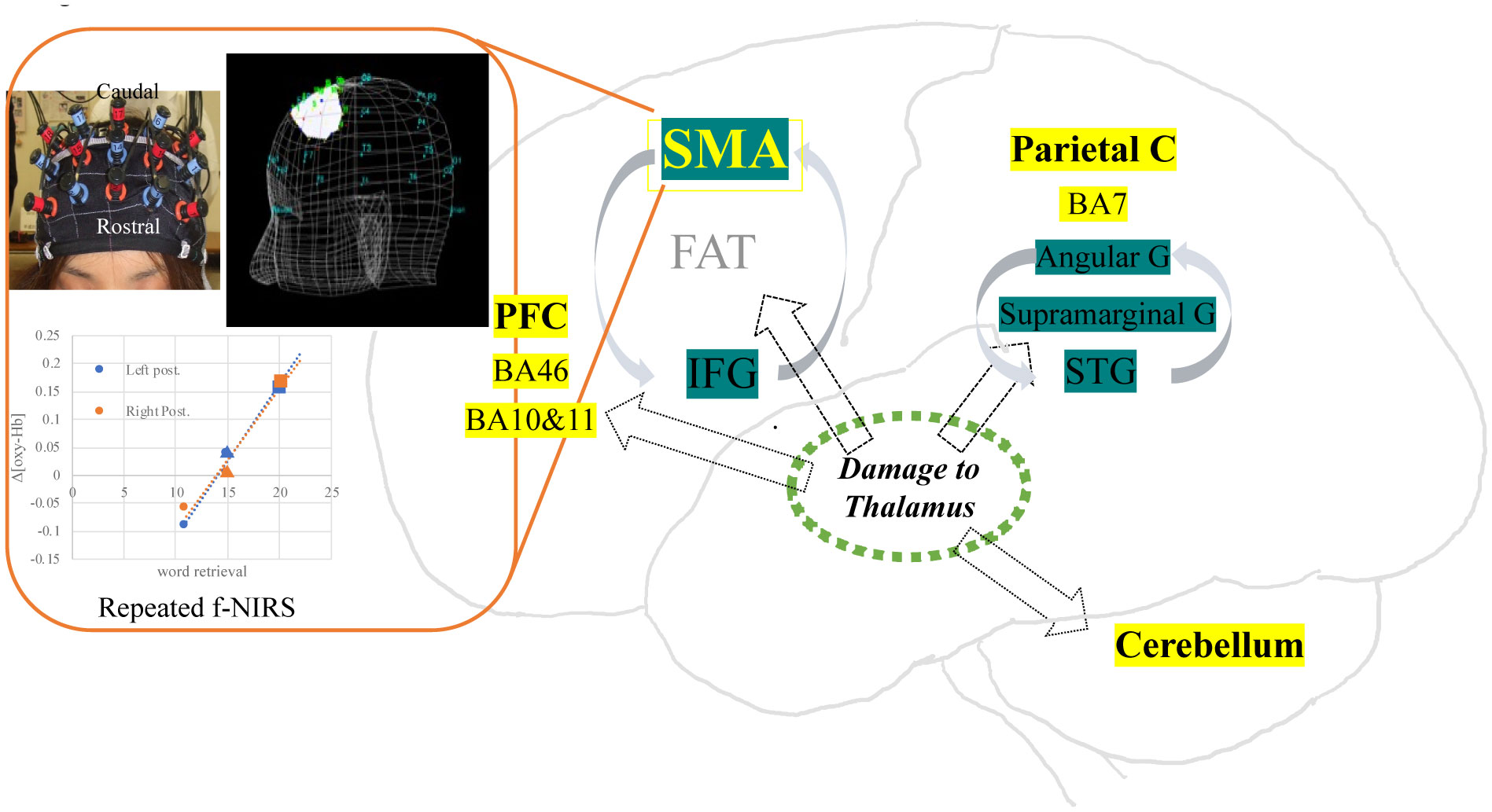
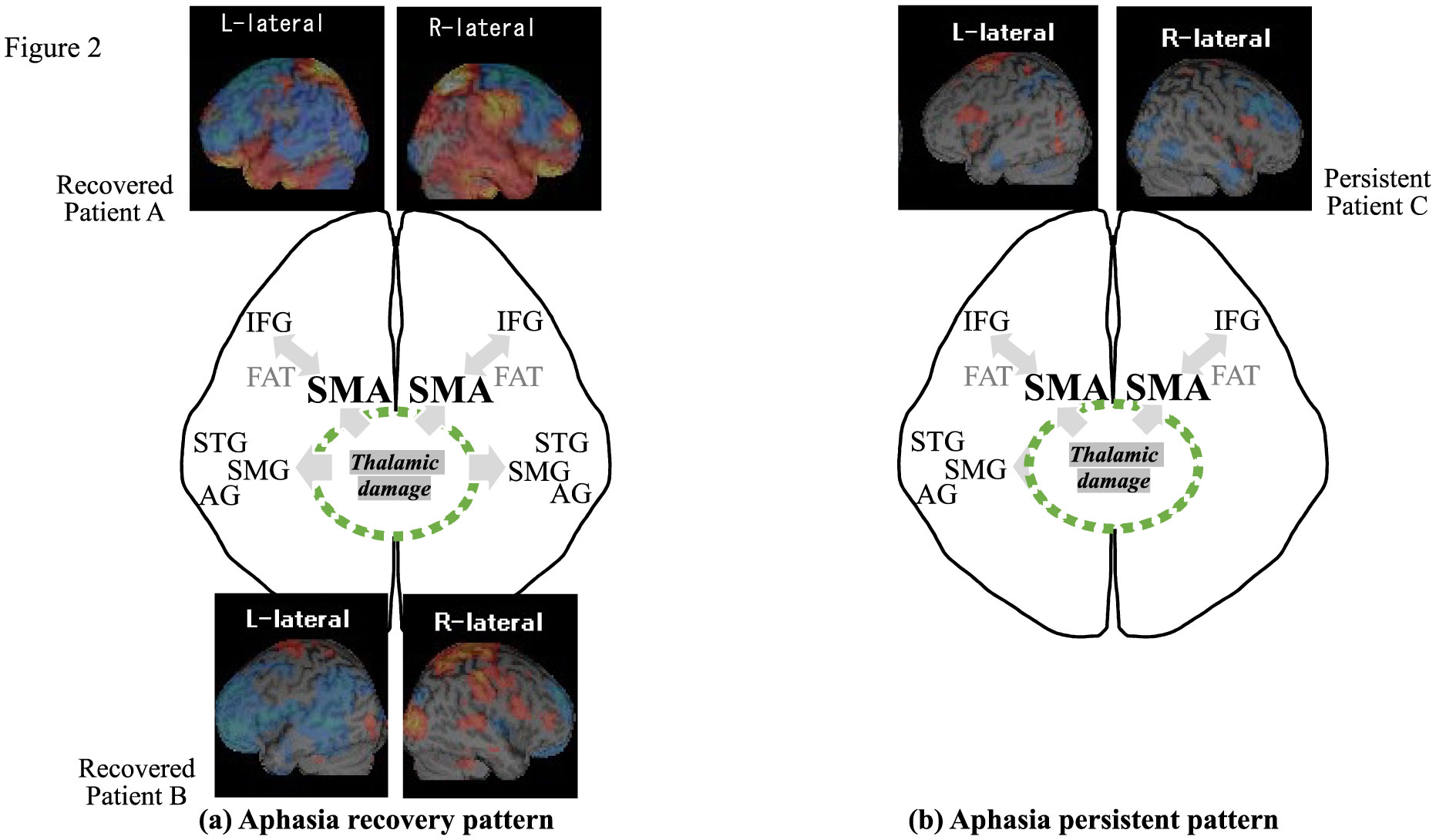
Thalamic stroke may result in cognitive and linguistic problems, but the underlying mechanism remains unknown. Especially, it is still a matter of debate why thalamic aphasia occasionally occurs and then mostly recovers to some degree. We begin with a brief overview of the cognitive dysfunction and aphasia, and then review previous hypotheses of the underlying mechanism. We introduced a unique characteristic of relatively transient “word retrieval difficulty” of patients in acute phase of thalamic stroke. Word retrieval ability involves both executive function and speech production. Furthermore, SMA aphasia and thalamic aphasia may resemble in terms of the rapid recovery, thus suggesting a shared neural system. This ability is attributable to the supplementary motor area (SMA) and inferior frontal cortex (IFG) via the frontal aslant tract (FAT). To explore the possible mechanism, we applied unique hybrid neuroimaging techniques: single-photon emission computed tomography (SPECT) and functional near-infrared spectroscopy (f-NIRS). SPECT can visualize the brain distribution associated with word retrieval difficulty, cognitive disability or aphasia after thalamic stroke, and f-NIRS focuses on SMA and monitors long-term changes in hemodynamic SMA responses during phonemic verbal task. SPECT yielded common perfusion abnormalities not only in the fronto–parieto–cerebellar–thalamic loop, but also in bilateral brain regions such as SMA, IFG and language-relevant regions. f-NIRS demonstrated that thalamic stroke developed significant word retrieval decline, which was intimately linked to posterior SMA responses. Word retrieval difficulty was rapidly recovered with increased bilateral SMA responses at follow-up NIRS. Together, we propose that the cognitive domain affected by thalamic stroke may be related to the fronto–parieto–cerebellar–thalamic loop, while the linguistic region may be attributable to SMA, IFG and language-related brain areas. Especially, bilateral SMA may play a crucial role in the recovery of word retrieval, and right language-related region, including IFG, angular gyrus and supramarginal gyrus may determine recovery from thalamic aphasia.

Abbreviations

angular gyrus

center median

FAT

frontal aslant tract

f-NIRS

functional near infrared spectroscopy

IFG

inferior frontal gyrus

ITP

inferior thalamic peduncle

nucleus reticularis thalami

PET

positron emission tomography

SMG

supramarginal gyrus

SMA

supplementary motor area

SPECT

single photon emission tomography

STG

superior temporal gyrus

Acknowledgments

This research was partially supported by a grant from Grants-in-Aid for Scientific Research, Japan Society for the Promotion of Science (JSPS) to S.O (19K11355).

Conflict of interest

The authors declare no conflict of interest.

References

[1]	Wolff M, Vann SD (2019) The Cognitive Thalamus as a Gateway to Mental Representations. J Neurosci 39: 3-14. https://doi.org/10.1523/JNEUROSCI.0479-18.2018. doi: 10.1523/JNEUROSCI.0479-18.2018
[2]	Valenstein E, Bowers D, Verfaellie M, et al. (1987) Retrosplenial amnesia. Brain 110: 1631-1646. https://doi.org/10.1093/brain/110.6.1631. doi: 10.1093/brain/110.6.1631
[3]	Aggleton JP, O'Mara SM, Vann SD, et al. (2010) Hippocampal-anterior thalamic pathways for memory: uncovering a network of direct and indirect actions. Eur J Neurosci 31: 2292-2307. https://doi.org/10.1111/j.1460-9568.2010.07251.x. doi: 10.1111/j.1460-9568.2010.07251.x
[4]	Van der Werf YD, Scheltens P, Lindeboom J, et al. (2003) Deficits of memory, executive functioning and attention following infarction in the thalamus; a study of 22 cases with localised lesions. Neuropsychologia 41: 1330-1344. https://doi.org/10.1016/S0028-3932(03)00059-9. doi: 10.1016/S0028-3932(03)00059-9
[5]	Carrera E, Bogousslavsky J (2006) The thalamus and behavior: effects of anatomically distinct strokes. Neurology 66: 1817-1823. https://doi.org/10.1212/01.wnl.0000219679.95223.4c. doi: 10.1212/01.wnl.0000219679.95223.4c
[6]	Johnson MD, Ojemann GA (2000) The role of the human thalamus in language and memory: evidence from electrophysiological studies. Brain Cogn 42: 218-230. https://doi.org/10.1006/brcg.1999.1101. doi: 10.1006/brcg.1999.1101
[7]	Crosson B (2013) Thalamic mechanisms in language: a reconsideration based on recent findings and concepts. Brain Lang 126: 73-88. https://doi.org/10.1016/j.bandl.2012.06.011. doi: 10.1016/j.bandl.2012.06.011
[8]	Raymer AM, Moberg P, Crosson B, et al. (1997) Lexical-semantic deficits in two patients with dominant thalamic infarction. Neuropsychologia 35: 211-219. https://doi.org/10.1016/S0028-3932(96)00069-3. doi: 10.1016/S0028-3932(96)00069-3
[9]	Demeurisse G, Derouck M, Coekaerts MJ, et al. (1979) Study of two cases of aphasia by infarction of the left thalamus, without cortical lesion. Acta Neurol Belg 79: 450-459.
[10]	Jonas S (1982) The thalamus and aphasia, including transcortical aphasia: a review. J Commun Disord 15: 31-41. https://doi.org/10.1016/0021-9924(82)90042-9. doi: 10.1016/0021-9924(82)90042-9
[11]	Llano DA (2013) Functional imaging of the thalamus in language. Brain Lang 126: 62-72. https://doi.org/10.1016/j.bandl.2012.06.004. doi: 10.1016/j.bandl.2012.06.004
[12]	Obayashi S (2020) The Supplementary Motor Area Responsible for Word Retrieval Decline After Acute Thalamic Stroke Revealed by Coupled SPECT and Near-Infrared Spectroscopy. Brain Sci 10: https://doi.org/10.3390/brainsci10040247. doi: 10.3390/brainsci10040247
[13]	De Witte L, Brouns R, Kavadias D, et al. (2011) Cognitive, affective and behavioural disturbances following vascular thalamic lesions: a review. Cortex 47: 273-319. https://doi.org/10.1016/j.cortex.2010.09.002. doi: 10.1016/j.cortex.2010.09.002
[14]	Nadeau SE, Crosson B (1997) Subcortical aphasia. Brain Lang 58: 355-402; discussion 418–323. https://doi.org/10.1006/brln.1997.1707. doi: 10.1006/brln.1997.1707
[15]	Fontaine D, Capelle L, Duffau H (2002) Somatotopy of the supplementary motor area: evidence from correlation of the extent of surgical resection with the clinical patterns of deficit. Neurosurgery 50: 297-303; discussion 303–295. https://doi.org/10.1227/00006123-200202000-00011.
[16]	Tremblay P, Gracco VL (2009) Contribution of the pre-SMA to the production of words and non-speech oral motor gestures, as revealed by repetitive transcranial magnetic stimulation (rTMS). Brain Research 1268: 112-124. https://doi.org/10.1016/j.brainres.2009.02.076. doi: 10.1016/j.brainres.2009.02.076
[17]	Alario FX, Chainay H, Lehericy S, et al. (2006) The role of the supplementary motor area (SMA) in word production. Brain Res 1076: 129-143. https://doi.org/10.1016/j.brainres.2005.11.104. doi: 10.1016/j.brainres.2005.11.104
[18]	Shima K, Mushiake H, Saito N, et al. (1996) Role for cells in the presupplementary motor area in updating motor plans. P Natl Acad Sci USA 93: 8694-8698. https://doi.org/10.1073/pnas.93.16.8694. doi: 10.1073/pnas.93.16.8694
[19]	Obayashi S, Hara Y (2013) Hypofrontal activity during word retrieval in older adults: a near-infrared spectroscopy study. Neuropsychologia 51: 418-424. https://doi.org/10.1016/j.neuropsychologia.2012.11.023. doi: 10.1016/j.neuropsychologia.2012.11.023
[20]	Catani M, Dell'acqua F, Vergani F, et al. (2012) Short frontal lobe connections of the human brain. Cortex 48: 273-291. https://doi.org/10.1016/j.cortex.2011.12.001. doi: 10.1016/j.cortex.2011.12.001
[21]	Thiebaut de Schotten M, Dell'Acqua F, Valabregue R, et al. (2012) Monkey to human comparative anatomy of the frontal lobe association tracts. Cortex 48: 82-96. https://doi.org/10.1016/j.cortex.2011.10.001. doi: 10.1016/j.cortex.2011.10.001
[22]	Dick AS, Garic D, Graziano P, et al. (2019) The frontal aslant tract (FAT) and its role in speech, language and executive function. Cortex 111: 148-163. https://doi.org/10.1016/j.cortex.2018.10.015. doi: 10.1016/j.cortex.2018.10.015
[23]	Costafreda SG, Fu CH, Lee L, et al. (2006) A systematic review and quantitative appraisal of fMRI studies of verbal fluency: role of the left inferior frontal gyrus. Hum Brain Mapp 27: 799-810. https://doi.org/10.1002/hbm.20221. doi: 10.1002/hbm.20221
[24]	Ziegler W, Kilian B, Deger K (1997) The role of the left mesial frontal cortex in fluent speech: evidence from a case of left supplementary motor area hemorrhage. Neuropsychologia 35: 1197-1208. https://doi.org/10.1016/S0028-3932(97)00040-7. doi: 10.1016/S0028-3932(97)00040-7
[25]	Ardila A, Lopez MV (1984) Transcortical motor aphasia: one or two aphasias? Brain Lang 22: 350-353. https://doi.org/10.1016/0093-934X(84)90099-3. doi: 10.1016/0093-934X(84)90099-3
[26]	Alexander MP, Schmitt MA (1980) The aphasia syndrome of stroke in the left anterior cerebral artery territory. Arch Neurol 37: 97-100. https://doi.org/10.1001/archneur.1980.00500510055010. doi: 10.1001/archneur.1980.00500510055010
[27]	Laplane D, Talairach J, Meininger V, et al. (1977) Clinical consequences of corticectomies involving the supplementary motor area in man. J Neurol Sci 34: 301-314. https://doi.org/10.1016/0022-510X(77)90148-4. doi: 10.1016/0022-510X(77)90148-4
[28]	Potgieser AR, de Jong BM, Wagemakers M, et al. (2014) Insights from the supplementary motor area syndrome in balancing movement initiation and inhibition. Front Hum Neurosci 8: 960https://doi.org/10.3389/fnhum.2014.00960. doi: 10.3389/fnhum.2014.00960
[29]	Kim YH, Kim CH, Kim JS, et al. (2013) Risk factor analysis of the development of new neurological deficits following supplementary motor area resection. J Neurosurg 119: 7-14. https://doi.org/10.3171/2013.3.JNS121492. doi: 10.3171/2013.3.JNS121492
[30]	Rosenberg K, Nossek E, Liebling R, et al. (2010) Prediction of neurological deficits and recovery after surgery in the supplementary motor area: a prospective study in 26 patients. J Neurosurg 113: 1152-1163. https://doi.org/10.3171/2010.6.JNS1090. doi: 10.3171/2010.6.JNS1090
[31]	Baker CM, Burks JD, Briggs RG, et al. (2018) The crossed frontal aslant tract: A possible pathway involved in the recovery of supplementary motor area syndrome. Brain Behav 8: e00926https://doi.org/10.1002/brb3.926. doi: 10.1002/brb3.926
[32]	Alario FX, Chainay H, Lehericy S, et al. (2006) The role of the supplementary motor area (SMA) in word production. Brain Res 1076: 129-143. https://doi.org/10.1016/j.brainres.2005.11.104. doi: 10.1016/j.brainres.2005.11.104
[33]	Obayashi S (2019) Frontal dynamic activity as a predictor of cognitive dysfunction after pontine ischemia. NeuroRehabilitation 44: 251-261. https://doi.org/10.3233/NRE-182566. doi: 10.3233/NRE-182566
[34]	Crosson B (1984) Role of the dominant thalamus in language: a review. Psychol Bull 96: 491-517. https://doi.org/10.1037/0033-2909.96.3.491. doi: 10.1037/0033-2909.96.3.491
[35]	Radanovic M, Scaff M (2003) Speech and language disturbances due to subcortical lesions. Brain Lang 84: 337-352. https://doi.org/10.1016/S0093-934X(02)00554-0. doi: 10.1016/S0093-934X(02)00554-0
[36]	Bell DS (1968) Speech functions of the thalamus inferred from the effects of thalamotomy. Brain 91: 619-638. https://doi.org/10.1093/brain/91.4.619. doi: 10.1093/brain/91.4.619
[37]	Levin N, Ben-Hur T, Biran I, et al. (2005) Category specific dysnomia after thalamic infarction: a case-control study. Neuropsychologia 43: 1385-1390. https://doi.org/10.1016/j.neuropsychologia.2004.12.001. doi: 10.1016/j.neuropsychologia.2004.12.001
[38]	Archer CR, Ilinsky IA, Goldfader PR, et al. (1981) Case report. Aphasia in thalamic stroke: CT stereotactic localization. J Comput Assist Tomogr 5: 427-432. https://doi.org/10.1097/00004728-198106000-00024. doi: 10.1097/00004728-198106000-00024
[39]	Karbe H, Thiel A, Weber-Luxenburger G, et al. (1998) Brain plasticity in poststroke aphasia: what is the contribution of the right hemisphere? Brain Lang 64: 215-230. https://doi.org/10.1006/brln.1998.1961. doi: 10.1006/brln.1998.1961
[40]	Calvert GA, Brammer MJ, Morris RG, et al. (2000) Using fMRI to study recovery from acquired dysphasia. Brain Lang 71: 391-399. https://doi.org/10.1006/brln.1999.2272. doi: 10.1006/brln.1999.2272
[41]	Saur D, Lange R, Baumgaertner A, et al. (2006) Dynamics of language reorganization after stroke. Brain 129: 1371-1384. https://doi.org/10.1093/brain/awl090. doi: 10.1093/brain/awl090
[42]	Anglade C, Thiel A, Ansaldo AI (2014) The complementary role of the cerebral hemispheres in recovery from aphasia after stroke: a critical review of literature. Brain Inj 28: 138-145. https://doi.org/10.3109/02699052.2013.859734. doi: 10.3109/02699052.2013.859734
[43]	Sebastian R, Long C, Purcell JJ, et al. (2016) Imaging network level language recovery after left PCA stroke. Restor Neurol Neurosci 34: 473-489. https://doi.org/10.3233/RNN-150621.

Reader Comments

Your name:*

Email:*
© 2022 the Author(s), licensee AIMS Press. This is an open access article distributed under the terms of the Creative Commons Attribution License (http://creativecommons.org/licenses/by/4.0)