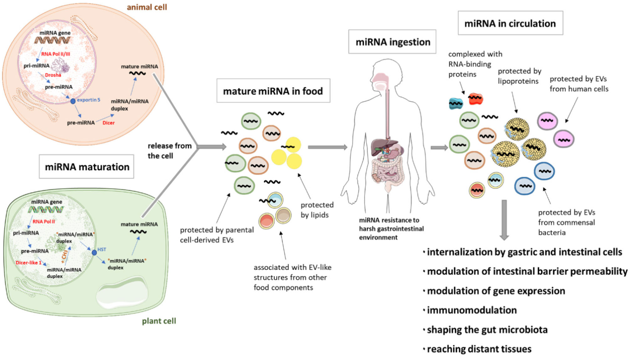
MicroRNAs (miRNAs), that is, short non-coding RNA molecules, have been found in different common foods, like fruits and vegetables, meat and its products, milk (including human breast milk) and dairy products, as well as honey and herbs. Moreover, they are isolated from supernatants from cultures of various mammalian cells. A growing amount of evidence appears to support the idea of using miRNAs as therapeutics. One possible and promising route of administration is oral, which is considered noninvasive and well-tolerated by patients. Association with extracellular vesicles (EVs), nanoparticles, RNA-binding proteins, lipoproteins, or lipid derivatives, protects miRNAs from an unfavorable gastrointestinal environment (including salivary and pancreatic RNases, low pH in the stomach, digestive enzymes, peristaltic activity and microbial enzymes). Such protection likely favors miRNA absorption from the digestive tract. Internalization of miRNA by gastric and intestinal cells as well as effects on the gut microbiota by orally delivered miRNA have recently been described. Furthermore, gene regulation by orally administered miRNAs and their immunomodulatory properties indicate the possibility of cross-species or cross-kingdom communication through miRNA. In addition to the local effects, these molecules may enter the circulatory system and reach distant tissues, and thus cell-free nucleic acids are promising candidates for future selective treatments of various diseases. Nonetheless, different limitations of such a therapy imply a number of questions for detailed investigation.
Citation: Martyna Cieślik, Krzysztof Bryniarski, Katarzyna Nazimek. Dietary and orally-delivered miRNAs: are they functional and ready to modulate immunity?[J]. AIMS Allergy and Immunology, 2023, 7(1): 104-131. doi: 10.3934/Allergy.2023008
MicroRNAs (miRNAs), that is, short non-coding RNA molecules, have been found in different common foods, like fruits and vegetables, meat and its products, milk (including human breast milk) and dairy products, as well as honey and herbs. Moreover, they are isolated from supernatants from cultures of various mammalian cells. A growing amount of evidence appears to support the idea of using miRNAs as therapeutics. One possible and promising route of administration is oral, which is considered noninvasive and well-tolerated by patients. Association with extracellular vesicles (EVs), nanoparticles, RNA-binding proteins, lipoproteins, or lipid derivatives, protects miRNAs from an unfavorable gastrointestinal environment (including salivary and pancreatic RNases, low pH in the stomach, digestive enzymes, peristaltic activity and microbial enzymes). Such protection likely favors miRNA absorption from the digestive tract. Internalization of miRNA by gastric and intestinal cells as well as effects on the gut microbiota by orally delivered miRNA have recently been described. Furthermore, gene regulation by orally administered miRNAs and their immunomodulatory properties indicate the possibility of cross-species or cross-kingdom communication through miRNA. In addition to the local effects, these molecules may enter the circulatory system and reach distant tissues, and thus cell-free nucleic acids are promising candidates for future selective treatments of various diseases. Nonetheless, different limitations of such a therapy imply a number of questions for detailed investigation.

| [1] |
Lu TX, Rothenberg ME (2018) MicroRNA. J Allergy Clin Immunol 141: 1202-1207. https://doi.org/10.1016/j.jaci.2017.08.034 
|
| [2] |
Bartel DP (2004) MicroRNAs. Cell 116: 281-297. https://doi.org/10.1016/S0092-8674(04)00045-5
|
| [3] |
Lee RC, Feinbaum RL, Ambros V (1993) The C. elegans heterochronic gene lin-4 encodes small RNAs with antisense complementarity to lin-14. Cell 75: 843-854. https://doi.org/10.1016/0092-8674(93)90529-Y
|
| [4] |
Ambros V (2004) The functions of animal microRNAs. Nature 431: 350-355. https://doi.org/10.1038/nature02871
|
| [5] |
Sikora E, Ptak W, Bryniarski K (2011) Immunoregulation by interference RNA (iRNA)—mechanisms, role, perspective. Postepy Hig Med Dosw 65: 482-495. https://doi.org/10.5604/17322693.954790
|
| [6] |
Serra F, Aielli L, Costantini E (2021) The role of miRNAs in the inflammatory phase of skin wound healing. AIMS Allergy Immunol 5: 264-278. https://doi.org/10.3934/Allergy.2021020
|
| [7] |
O'Brien J, Hayder H, Zayed Y, et al. (2018) Overview of microRNA biogenesis, mechanisms of actions, and circulation. Front Endocrinol 9: 402. https://doi.org/10.3389/fendo.2018.00402
|
| [8] |
Chekulaeva M, Filipowicz W (2009) Mechanisms of miRNA-mediated post-transcriptional regulation in animal cells. Curr Opin Cell Biol 21: 452-460. https://doi.org/10.1016/j.ceb.2009.04.009
|
| [9] |
Jame-Chenarboo F, Ng HH, Macdonald D, et al. (2022) High-throughput analysis reveals miRNA upregulating α-2,6-sialic acid through direct miRNA–mRNA interactions. ACS Cent Sci 8: 1527-1536. https://doi.org/10.1021/acscentsci.2c00748
|
| [10] |
Boon RA, Vickers KC (2013) Intercellular transport of microRNAs. Arterioscl Throm Vas 33: 186-192. https://doi.org/10.1161/ATVBAHA.112.300139
|
| [11] | Pogue AI, Clement C, Hill JM, et al. (2014) Evolution of microRNA (miRNA) structure and function in plants and animals: Relevance to aging and disease. J Aging Sci 2: 119. |
| [12] |
Chen X, Liang H, Zhang J, et al. (2012) Horizontal transfer of microRNAs: molecular mechanisms and clinical applications. Protein Cell 3: 28-37. https://doi.org/10.1007/s13238-012-2003-z
|
| [13] |
Wang K, Zhang S, Weber J, et al. (2010) Export of microRNAs and microRNA-protective protein by mammalian cells. Nucleic Acids Res 38: 7248-7259. https://doi.org/10.1093/nar/gkq601
|
| [14] |
Turchinovich A, Weiz L, Langheinz A, et al. (2011) Characterization of extracellular circulating microRNA. Nucleic Acids Res 39: 7223-7233. https://doi.org/10.1093/nar/gkr254
|
| [15] |
Gallo A, Tandon M, Alevizos I, et al. (2012) The majority of microRNAs detectable in serum and saliva is concentrated in exosomes. PLoS One 7: e30679. https://doi.org/10.1371/journal.pone.0030679
|
| [16] |
Kosaka N, Iguchi H, Yoshioka Y, et al. (2010) Secretory mechanisms and intercellular transfer of microRNAs in living cells. J Biol Chem 285: 17442-17452. https://doi.org/10.1074/jbc.M110.107821
|
| [17] |
Meister G, Landthaler M, Patkaniowska A, et al. (2004) Human Argonaute2 mediates RNA cleavage targeted by miRNAs and siRNAs. Mol Cell 15: 185-197. https://doi.org/10.1016/j.molcel.2004.07.007
|
| [18] |
Winter J, Jung S, Keller S, et al. (2009) Many roads to maturity: microRNA biogenesis pathways and their regulation. Nat Cell Biol 11: 228-234. https://doi.org/10.1038/ncb0309-228
|
| [19] |
Hutvagner G, Simard MJ (2008) Argonaute proteins: key players in RNA silencing. Nat Rev Mol Cell Bio 9: 22-32. https://doi.org/10.1038/nrm2321
|
| [20] |
Czech B, Hannon GJ (2011) Small RNA sorting: matchmaking for Argonautes. Nat Rev Genet 12: 19-31. https://doi.org/10.1038/nrg2916
|
| [21] |
Sedgeman LR, Beysen C, Solano MAR, et al. (2019) Beta cell secretion of miR-375 to HDL is inversely associated with insulin secretion. Sci Rep 9: 3803. https://doi.org/10.1038/s41598-019-40338-7
|
| [22] |
Vickers KC, Palmisano BT, Shoucri BM, et al. (2011) MicroRNAs are transported in plasma and delivered to recipient cells by high-density lipoproteins. Nat Cell Biol 13: 423-433. https://doi.org/10.1038/ncb2210
|
| [23] |
Tabet F, Vickers KC, Torres LFC, et al. (2014) HDL-transferred microRNA-223 regulates ICAM-1 expression in endothelial cells. Nat Commun 5: 3292. https://doi.org/10.1038/ncomms4292
|
| [24] |
Michell DL, Vickers KC (2016) Lipoprotein carriers of microRNAs. Biochim Biophys Acta 1861: 2069-2074. https://doi.org/10.1016/j.bbalip.2016.01.011
|
| [25] |
Askenase PW (2021) Exosomes provide unappreciated carrier effects that assist transfers of their miRNAs to targeted cells; I. They are ‘The Elephant in the Room’. RNA Biol 18: 2038-2053. https://doi.org/10.1080/15476286.2021.1885189
|
| [26] |
del Pozo-Acebo L, de las Hazas MCL, Tomé-Carneiro J, et al. (2021) Bovine milk-derived exosomes as a drug delivery vehicle for miRNA-based therapy. Int J Mol Sci 22: 1105. https://doi.org/10.3390/ijms22031105
|
| [27] |
Matsuzaka Y, Yashiro R (2022) Immune modulation using extracellular vesicles encapsulated with microRNAs as novel drug delivery systems. Int J Mol Sci 23: 5658. https://doi.org/10.3390/ijms23105658
|
| [28] |
Das CK, Jena BC, Banerjee I, et al. (2019) Exosome as a novel shuttle for delivery of therapeutics across biological barriers. Mol Pharmacol 16: 24-40. https://doi.org/10.1021/acs.molpharmaceut.8b00901
|
| [29] |
Hachimura S, Totsuka M, Hosono A (2018) Immunomodulation by food: impact on gut immunity and immune cell function. Biosci Biotech Bioch 82: 584-599. https://doi.org/10.1080/09168451.2018.1433017
|
| [30] |
Wagner AE, Piegholdt S, Ferraro M, et al. (2015) Food derived microRNAs. Food Funct 6: 714-718. https://doi.org/10.1039/C4FO01119H
|
| [31] |
Zempleni J, Baier SR, Howard KM, et al. (2015) Gene regulation by dietary microRNAs. Can J Physiol Pharm 93: 1097-1102. https://doi.org/10.1139/cjpp-2014-0392
|
| [32] |
Cui J, Zhou B, Ross SA, et al. (2017) Nutrition, microRNAs, and human health. Adv Nutr 8: 105-112. https://doi.org/10.3945/an.116.013839
|
| [33] |
Li X, Qi L (2022) Epigenetics in precision nutrition. J Pers Med 12: 533. https://doi.org/10.3390/jpm12040533
|
| [34] |
Witzany G (2012) Do we eat gene regulators?. Commun Integr Biol 5: 230-232. https://doi.org/10.4161/cib.19621
|
| [35] |
Zhu R, Zhang Z, Li Y, et al. (2016) Discovering numerical differences between animal and plant microRNAs. PLoS One 11: e0165152. https://doi.org/10.1371/journal.pone.0165152
|
| [36] |
Pradillo M, Santos JL (2018) Genes involved in miRNA biogenesis affect meiosis and fertility. Chromosome Res 26: 233-241. https://doi.org/10.1007/s10577-018-9588-x
|
| [37] |
Yu B, Yang Z, Li J, et al. (2005) Methylation as a crucial step in plant microRNA biogenesis. Science 307: 932-935. https://doi.org/10.1126/science.1107130
|
| [38] |
Ji L, Chen X (2012) Regulation of small RNA stability: methylation and beyond. Cell Res 22: 624-636. https://doi.org/10.1038/cr.2012.36
|
| [39] |
Wang X, Ren X, Ning L, et al. (2020) Stability and absorption mechanism of typical plant miRNAs in an in vitro gastrointestinal environment: basis for their cross-kingdom nutritional effects. J Nutr Biochem 81: 108376. https://doi.org/10.1016/j.jnutbio.2020.108376
|
| [40] |
Zhao Y, Mo B, Chen X (2012) Mechanisms that impact microRNA stability in plants. RNA Biol 9: 1218-1223. https://doi.org/10.4161/rna.22034
|
| [41] |
Millar AA, Waterhouse PM (2005) Plant and animal microRNAs: similarities and differences. Funct Integr Genomics 5: 129-135. https://doi.org/10.1007/s10142-005-0145-2
|
| [42] |
Carrington JC, Ambros V (2003) Role of microRNAs in plant and animal development. Science 301: 336-338. https://doi.org/10.1126/science.1085242
|
| [43] |
Arteaga-Vázquez M, Caballero-Pérez J, Vielle-Calzada JP (2007) A family of microRNAs present in plants and animals. Plant Cell 18: 3355-3369. https://doi.org/10.1105/tpc.106.044420
|
| [44] |
Li J, Lei L, Ye F, et al. (2019) Nutritive implications of dietary microRNAs: facts, controversies, and perspectives. Food Funct 10: 3044-3056. https://doi.org/10.1039/C9FO00216B
|
| [45] |
Rosenthal KS, Baker JB (2022) The immune system through the ages. AIMS Allergy Immunol 6: 170-187. https://doi.org/10.3934/Allergy.2022013
|
| [46] |
Hatmal MM, Al-Hatamleh MAI, Olaimat AN, et al. (2022) Immunomodulatory properties of human breast milk: MicroRNA contents and potential epigenetic effects. Biomedicines 10: 1219. https://doi.org/10.3390/biomedicines10061219
|
| [47] |
Kosaka N, Izumi H, Sekine K, et al. (2010) MicroRNA as a new immune-regulatory agent in breast milk. Silence 1: 7. https://doi.org/10.1186/1758-907X-1-7
|
| [48] |
Zhou Q, Li M, Wang X, et al. (2012) Immune-related microRNAs are abundant in breast milk exosomes. Int J Biol Sci 8: 118-123. https://doi.org/10.7150/ijbs.8.118
|
| [49] |
Vélez-Ixta JM, Benítez-Guerrero T, Aguilera-Hernández A, et al. (2022) Detection and quantification of immunoregulatory miRNAs in human milk and infant milk formula. BioTech 11: 11. https://doi.org/10.3390/biotech11020011
|
| [50] |
Chiba T, Kooka A, Kowatari K, et al. (2022) Expression profiles of hsa-miR-148a-3p and hsa-miR-125b-5p in human breast milk and infant formulae. Int Breastfeed J 17: 1. https://doi.org/10.1186/s13006-021-00436-7
|
| [51] |
Munch EM, Harris RA, Mohammad M, et al. (2013) Transcriptome profiling of microRNA by next-gen deep sequencing reveals known and novel miRNA species in the lipid fraction of human breast milk. PLoS One 8: e50564. https://doi.org/10.1371/journal.pone.0050564
|
| [52] |
Alsaweed M, Lai CT, Hartmann PE, et al. (2016) Human milk cells and lipids conserve numerous known and novel miRNAs, some of which are differentially expressed during lactation. PLoS One 11: e0152610. https://doi.org/10.1371/journal.pone.0152610
|
| [53] |
Floris I, Billard H, Boquien CY, et al. (2015) MiRNA analysis by quantitative PCR in preterm human breast milk reveals daily fluctuations of hsa-miR-16-5p. PLoS One 10: e0140488. https://doi.org/10.1371/journal.pone.0140488
|
| [54] |
Hicks SD, Confair A, Warren K, et al. (2021) Levels of breast milk microRNAs and other non-coding RNAs are impacted by milk maturity and maternal diet. Front Immunol 12: 785217. https://doi.org/10.3389/fimmu.2021.785217
|
| [55] |
Gregg B, Ellsworth L, Pavela G, et al. (2022) Bioactive compounds in mothers milk affecting offspring outcomes: A narrative review. Pediatr Obes 17: e12892. https://doi.org/10.1111/ijpo.12892
|
| [56] |
van Herwijnen MJC, Driedonks TAP, Snoek BL, et al. (2018) Abundantly present miRNAs in milk-derived extracellular vesicles are conserved between mammals. Front Nutr 5: 81. https://doi.org/10.3389/fnut.2018.00081
|
| [57] |
Wang H, Wu D, Sukreet S, et al. (2022) Quantitation of exosomes and their microRNA cargos in frozen human milk. JPGN Rep 3: e172. https://doi.org/10.1097/PG9.0000000000000172
|
| [58] |
Chutipongtanate S, Morrow AL, Newburg DS (2022) Human milk extracellular vesicles: A biological system with clinical implications. Cells 11: 2345. https://doi.org/10.3390/cells11152345
|
| [59] |
Golan-Gerstl R, Reif S (2022) Extracellular vesicles in human milk. Curr Opin Clin Nutr Metab Care 25: 209-215. https://doi.org/10.1097/MCO.0000000000000834
|
| [60] |
Aarts J, Boleij A, Pieters BCH, et al. (2021) Flood control: How milk-derived extracellular vesicles can help to improve the intestinal barrier function and break the gut-joint axis in rheumatoid arthritis. Front Immunol 12: 703277. https://doi.org/10.3389/fimmu.2021.703277
|
| [61] |
Kupsco A, Lee JJ, Prada D, et al. (2022) Marine pollutant exposures and human milk extracellular vesicle-microRNAs in a mother-infant cohort from the Faroe Islands. Environ Int 158: 106986. https://doi.org/10.1016/j.envint.2021.106986
|
| [62] |
Alsaweed M, Lai CT, Hartmann PE, et al. (2016) Human milk miRNAs primarily originate from the mammary gland resulting in unique miRNA profiles of fractionated milk. Sci Rep 6: 20680. https://doi.org/10.1038/srep20680
|
| [63] |
Chen X, Gao C, Li H, et al. (2010) Identification and characterization of microRNAs in raw milk during different periods of lactation, commercial fluid, and powdered milk products. Cell Res 20: 1128-1137. https://doi.org/10.1038/cr.2010.80
|
| [64] |
Izumi H, Kosaka N, Shimizu T, et al. (2012) Bovine milk contains microRNA and messenger RNA that are stable under degradative conditions. J Dairy Sci 95: 4831-4841. https://doi.org/10.3168/jds.2012-5489
|
| [65] |
Hata T, Murakami K, Nakatani H, et al. (2010) Isolation of bovine milk-derived microvesicles carrying mRNAs and microRNAs. Biochem Biophys Res Commun 396: 528-533. https://doi.org/10.1016/j.bbrc.2010.04.135
|
| [66] |
Benmoussa A, Laugier J, Beauparlant CJ, et al. (2020) Complexity of the microRNA transcriptome of cow milk and milk-derived extracellular vesicles isolated via differential ultracentrifugation. J Dairy Sci 103: 16-29. https://doi.org/10.3168/jds.2019-16880
|
| [67] |
Li R, Dudemaine PL, Zhao X, et al. (2016) Comparative analysis of the miRNome of bovine milk fat, whey and cells. PLoS One 11: e0154129. https://doi.org/10.1371/journal.pone.0154129
|
| [68] |
Cui X, Zhang S, Zhang Q, et al. (2020) Comprehensive microRNA expression profile of the mammary gland in lactating dairy cows with extremely different milk protein and fat percentages. Front Genet 11: 548268. https://doi.org/10.3389/fgene.2020.548268
|
| [69] |
Cai W, Li C, Li J, et al. (2021) Integrated small RNA sequencing, transcriptome and GWAS data reveal microrna regulation in response to milk protein traits in chinese holstein cattle. Front Genet 12: 726706. https://doi.org/10.3389/fgene.2021.726706
|
| [70] |
Shome S, Jernigan RL, Beitz DC, et al. (2021) Non-coding RNA in raw and commercially processed milk and putative targets related to growth and immune-response. BMC Genomics 22: 749. https://doi.org/10.1186/s12864-021-07964-w
|
| [71] |
Zhang Y, Xu Q, Hou J, et al. (2022) Loss of bioactive microRNAs in cow's milk by ultra-high-temperature treatment but not by pasteurization treatment. J Sci Food Agric 102: 2676-2685. https://doi.org/10.1002/jsfa.11607
|
| [72] |
Yun B, Kim Y, Park DJ, et al. (2021) Comparative analysis of dietary exosome-derived microRNAs from human, bovine and caprine colostrum and mature milk. J Anim Sci Technol 63: 593-602. https://doi.org/10.5187/jast.2021.e39
|
| [73] |
Mecocci S, Pietrucci D, Milanesi M, et al. (2021) Transcriptomic characterization of cow, donkey and goat milk extracellular vesicles reveals their anti-inflammatory and immunomodulatory potential. Int J Mol Sci 22: 12759. https://doi.org/10.3390/ijms222312759
|
| [74] |
Izumi H, Tsuda M, Sato Y, et al. (2015) Bovine milk exosomes contain microRNA and mRNA and are taken up by human macrophages. J Dairy Sci 98: 2920-2933. https://doi.org/10.3168/jds.2014-9076
|
| [75] |
Benmoussa A, Provost P (2019) Milk microRNAs in health and disease. Compr Rev Food Sci Food Saf 18: 703-722. https://doi.org/10.1111/1541-4337.12424
|
| [76] |
Wehbe Z, Kreydiyyeh S (2022) Cow's milk may be delivering potentially harmful undetected cargoes to humans. Is it time to reconsider dairy recommendations?. Nutr Rev 80: 874-888. https://doi.org/10.1093/nutrit/nuab046
|
| [77] |
Wade B, Cummins M, Keyburn A, et al. (2016) Isolation and detection of microRNA from the egg of chickens. BMC Res Notes 9: 283. https://doi.org/10.1186/s13104-016-2084-5
|
| [78] |
Link J, Thon C, Schanze D, et al. (2019) Food-derived xeno-microRNAs: Influence of diet and detectability in gastrointestinal tract—proof-of-principle study. Mol Nutr Food Res 63: e1800076. https://doi.org/10.1002/mnfr.201800076
|
| [79] |
Dever JT, Kemp MQ, Thompson AL, et al. (2015) Survival and diversity of human homologous dietary micrornas in conventionally cooked top sirloin and dried bovine tissue extracts. PLoS One 10: e0138275. https://doi.org/10.1371/journal.pone.0138275
|
| [80] |
Gismondi A, Di Marco G, Canini A (2017) Detection of plant microRNAs in honey. PLoS One 12: e0172981. https://doi.org/10.1371/journal.pone.0172981
|
| [81] | Smith C, Cokcetin N, Truong T, et al. (2021) Cataloguing the small RNA content of honey using next generation sequencing. Food Chem 2: 100014. https://doi.org/10.1016/j.fochms.2021.100014 |
| [82] | Chen X, Liu B, Li X, et al. (2021) Identification of anti-inflammatory vesicle-like nanoparticles in honey. J Extracell Vesicles 10: e12069. https://doi.org/10.1002/jev2.12069 |
| [83] |
Gharehdaghi L, Bakhtiarizadeh MR, He K, et al. (2021) Diet-derived transmission of microRNAs from host plant into honey bee Midgut. BMC Genomics 22: 587. https://doi.org/10.1186/s12864-021-07916-4
|
| [84] |
Mu J, Zhuang X, Wang Q, et al. (2014) Interspecies communication between plant and mouse gut host cells through edible plant derived exosome-like nanoparticles. Mol Nutr Food Res 58: 1561-1573. https://doi.org/10.1002/mnfr.201300729
|
| [85] |
Cavallini A, Minervini F, Garbetta A, et al. (2018) High degradation and no bioavailability of artichoke miRNAs assessed using an in vitro digestion/Caco-2 cell model. Nutr Res 60: 68-76. https://doi.org/10.1016/j.nutres.2018.08.007
|
| [86] |
Lukasik A, Zielenkiewicz P (2014) In silico identification of plant miRNAs in mammalian breast milk exosomes—A small step forward?. PLoS One 9: e99963. https://doi.org/10.1371/journal.pone.0099963
|
| [87] |
Liang G, Zhu Y, Sun B, et al. (2014) Assessing the survival of exogenous plant microRNA in mice. Food Sci Nutr 2: 380-388. https://doi.org/10.1002/fsn3.113
|
| [88] |
Xiao J, Feng S, Wang X, et al. (2018) Identification of exosome-like nanoparticle-derived microRNAs from 11 edible fruits and vegetables. PeerJ 6: e5186. https://doi.org/10.7717/peerj.5186
|
| [89] |
Huang H, Pham Q, Davis CD, et al. (2020) Delineating effect of corn microRNAs and matrix, ingested as whole food, on gut microbiota in a rodent model. Food Sci Nutr 8: 4066-4077. https://doi.org/10.1002/fsn3.1672
|
| [90] |
Luo Y, Wang P, Wang X, et al. (2017) Detection of dietetically absorbed maize-derived microRNAs in pigs. Sci Rep 7: 645. https://doi.org/10.1038/s41598-017-00488-y
|
| [91] |
Liang H, Zhang S, Fu Z, et al. (2015) Effective detection and quantification of dietetically absorbed plant microRNAs in human plasma. J Nutr Biochem 26: 505-512. https://doi.org/10.1016/j.jnutbio.2014.12.002
|
| [92] |
Tomé-Carneiro J, Fernández-Alonso N, Tomás-Zapico C, et al. (2018) Breast milk microRNAs harsh journey towards potential effects in infant development and maturation. Lipid encapsulation can help. Pharmacol Res 132: 21-32. https://doi.org/10.1016/j.phrs.2018.04.003
|
| [93] |
del Pozo-Acebo L, de las Hazas MCL, Margollés A, et al. (2021) Eating microRNAs: pharmacological opportunities for cross-kingdom regulation and implications in host gene and gut microbiota modulation. Brit J Pharmacol 178: 2218-2245. https://doi.org/10.1111/bph.15421
|
| [94] |
Mar-Aguilar F, Arreola-Triana A, Mata-Cardona D, et al. (2020) Evidence of transfer of miRNAs from the diet to the blood still inconclusive. PeerJ 8: e9567. https://doi.org/10.7717/peerj.9567
|
| [95] |
Manca S, Upadhyaya B, Mutai E, et al. (2018) Milk exosomes are bioavailable and distinct microRNA cargos have unique tissue distribution patterns. Sci Rep 8: 11321. https://doi.org/10.1038/s41598-018-29780-1
|
| [96] |
Umezu T, Takanashi M, Murakami Y, et al. (2021) Acerola exosome-like nanovesicles to systemically deliver nucleic acid medicine via oral administration. Mol Ther Methods Clin Dev 21: 199-208. https://doi.org/10.1016/j.omtm.2021.03.006
|
| [97] |
Wiklander OPB, Nordin JZ, O'Loughlin A, et al. (2015) Extracellular vesicle in vivo biodistribution is determined by cell source, route of administration and targeting. J Extracell Vesicles 4: 26316. https://doi.org/10.3402/jev.v4.26316
|
| [98] |
Pieri M, Theori E, Dweep H, et al. (2022) A bovine miRNA, bta-miR-154c, withstands in vitro human digestion but does not affect cell viability of colorectal human cell lines after transfection. FEBS Open Bio 12: 925-936. https://doi.org/10.1002/2211-5463.13402
|
| [99] |
Baier SR, Nguyen C, Xie F, et al. (2014) MicroRNAs are absorbed in biologically meaningful amounts from nutritionally relevant doses of cow milk and affect gene expression in peripheral blood mononuclear cells, HEK-293 kidney cell cultures, and mouse livers. J Nutr 144: 1495-1500. https://doi.org/10.3945/jn.114.196436
|
| [100] |
Baier S, Howard K, Cui J, et al. (2015) MicroRNAs in chicken eggs are bioavailable in healthy adults and can modulate mRNA expression in peripheral blood mononuclear cells. FASEB J 29: LB322. https://doi.org/10.1096/fasebj.29.1_supplement.lb322
|
| [101] |
de las Hazas MCL, del Pozo-Acebo L, Hansen MS, et al. (2022) Dietary bovine milk miRNAs transported in extracellular vesicles are partially stable during GI digestion, are bioavailable and reach target tissues but need a minimum dose to impact on gene expression. Eur J Nutr 61: 1043-1056. https://doi.org/10.1007/s00394-021-02720-y
|
| [102] |
Beuzelin D, Pitard B, Kaeffer B (2019) Oral delivery of mirna with lipidic aminoglycoside derivatives in the breastfed rat. Front Physiol 10: 1037. https://doi.org/10.3389/fphys.2019.01037
|
| [103] |
Lin D, Chen T, Xie M, et al. (2020) Oral administration of bovine and porcine milk exosome alter miRNAs profiles in piglet serum. Sci Rep 10: 6983. https://doi.org/10.1038/s41598-020-63485-8
|
| [104] |
Zhou F, Ebea P, Mutai E, et al. (2022) Small extracellular vesicles in milk cross the blood-brain barrier in murine cerebral cortex endothelial cells and promote dendritic complexity in the hippocampus and brain function in C57BL/6J mice. Front Nutr 9: 838543. https://doi.org/10.3389/fnut.2022.838543
|
| [105] |
Rani P, Vashisht M, Golla N, et al. (2017) Milk miRNAs encapsulated in exosomes are stable to human digestion and permeable to intestinal barrier in vitro. J Funct Foods 34: 431-439. https://doi.org/10.1016/j.jff.2017.05.009
|
| [106] |
Liao Y, Du X, Li J, et al. (2017) Human milk exosomes and their microRNAs survive digestion in vitro and are taken up by human intestinal cells. Mol Nutr Food Res 61: 1700082. https://doi.org/10.1002/mnfr.201700082
|
| [107] |
Kahn S, Liao Y, Du X, et al. (2018) Exosomal microRNAs in milk from mothers delivering preterm infants survive in vitro digestion and are taken up by human intestinal cells. Mol Nutr Food Res 62: 1701050. https://doi.org/10.1002/mnfr.201701050
|
| [108] |
Liu YC, Chen WL, Kung WH, et al. (2017) Plant miRNAs found in human circulating system provide evidences of cross kingdom RNAi. BMC Genomics 18: 112. https://doi.org/10.1186/s12864-017-3502-3
|
| [109] |
Zhang L, Hou D, Chen X, et al. (2012) Exogenous plant MIR168a specifically targets mammalian LDLRAP1: evidence of cross-kingdom regulation by microRNA. Cell Res 22: 107-126. https://doi.org/10.1038/cr.2011.158
|
| [110] |
Yang J, Farmer LM, Agyekum AA, et al. (2015) Detection of dietary plant-based small RNAs in animals. Cell Res 25: 517-520. https://doi.org/10.1038/cr.2015.26
|
| [111] |
Yang J, Farmer LM, Agyekum AAA, et al. (2015) Detection of an abundant plant-based small RNA in healthy consumers. PLoS One 10: e0137516. https://doi.org/10.1371/journal.pone.0137516
|
| [112] |
Witwer KW, McAlexander MA, Queen SE, et al. (2013) Real-time quantitative PCR and droplet digital PCR for plant miRNAs in mammalian blood provide little evidence for general uptake of dietary miRNAs: Limited evidence for general uptake of dietary plant xenomiRs. RNA Biol 10: 1080-1086. https://doi.org/10.4161/rna.25246
|
| [113] |
Snow JW, Hale AE, Isaacs SK, et al. (2013) Ineffective delivery of diet-derived microRNAs to recipient animal organisms. RNA Biol 10: 1107-1116. https://doi.org/10.4161/rna.24909
|
| [114] |
Masood M, Everett CP, Chan SY, et al. (2016) Negligible uptake and transfer of diet-derived pollen microRNAs in adult honey bees. RNA Biol 13: 109-118. https://doi.org/10.1080/15476286.2015.1128063
|
| [115] |
Huang H, Davis CD, Wang TTY (2018) Extensive degradation and low bioavailability of orally consumed corn miRNAs in mice. Nutrients 10: E215. https://doi.org/10.3390/nu10020215
|
| [116] |
Qin X, Wang X, Xu K, et al. (2022) Digestion of plant dietary miRNAs starts in the mouth under the protection of coingested food components and plant-derived exosome-like nanoparticles. J Agr Food Chem 70: 4316-4327. https://doi.org/10.1021/acs.jafc.1c07730
|
| [117] |
Philip A, Ferro VA, Tate RJ (2015) Determination of the potential bioavailability of plant microRNAs using a simulated human digestion process. Mol Nutr Food Res 59: 1962-1972. https://doi.org/10.1002/mnfr.201500137
|
| [118] |
Bryniarski K, Ptak W, Martin E, et al. (2015) Free extracellular miRNA functionally targets cells by transfecting exosomes from their companion cells. PLoS One 10: e0122991. https://doi.org/10.1371/journal.pone.0122991
|
| [119] |
Li D, Yao X, Yue J, et al. (2022) Advances in bioactivity of microRNAs of plant-derived exosome-like nanoparticles and milk-derived extracellular vesicles. J Agr Food Chem 70: 6285-6299. https://doi.org/10.1021/acs.jafc.2c00631
|
| [120] |
Jia M, He J, Bai W, et al. (2021) Cross-kingdom regulation by dietary plant miRNAs: an evidence-based review with recent updates. Food Funct 12: 9549-9562. https://doi.org/10.1039/D1FO01156A
|
| [121] |
McKernan DP (2019) Toll-like receptors and immune cell crosstalk in the intestinal epithelium. AIMS Allergy Immunol 3: 13-31. https://doi.org/10.3934/Allergy.2019.1.13
|
| [122] |
Fritz JV, Heintz-Buschart A, Ghosal A, et al. (2016) Sources and functions of extracellular small RNAs in human circulation. Annu Rev Nutr 36: 301-336. https://doi.org/10.1146/annurev-nutr-071715-050711
|
| [123] |
Chen Q, Zhang F, Dong L, et al. (2021) SIDT1-dependent absorption in the stomach mediates host uptake of dietary and orally administered microRNAs. Cell Res 31: 247-258. https://doi.org/10.1038/s41422-020-0389-3
|
| [124] |
Cieślik M, Nazimek K, Bryniarski K (2022) Extracellular vesicles—Oral therapeutics of the future. Int J Mol Sci 23: 7554. https://doi.org/10.3390/ijms23147554
|
| [125] |
Carobolante G, Mantaj J, Ferrari E, et al. (2020) Cow milk and intestinal epithelial cell-derived extracellular vesicles as systems for enhancing oral drug delivery. Pharmaceutics 12: 226. https://doi.org/10.3390/pharmaceutics12030226
|
| [126] |
Akuma P, Okagu OD, Udenigwe CC (2019) Naturally occurring exosome vesicles as potential delivery vehicle for bioactive compounds. Front Sustain Food Syst 3: 23. https://doi.org/10.3389/fsufs.2019.00023
|
| [127] |
Zhang Y, Li J, Gao W, et al. (2022) Exosomes as anticancer drug delivery vehicles: Prospects and challenges. Front Biosci 27: 293. https://doi.org/10.31083/j.fbl2710293
|
| [128] |
Somiya M (2020) Where does the cargo go? Solutions to provide experimental support for the “extracellular vesicle cargo transfer hypothesis”. J Cell Commun Signal 14: 135-146. https://doi.org/10.1007/s12079-020-00552-9
|
| [129] |
Askenase PW (2022) Exosome carrier effects; resistance to digestion in phagolysosomes may assist transfers to targeted cells; II transfers of miRNAs are better analyzed via systems approach as they do not fit conventional reductionist stoichiometric concepts. Int J Mol Sci 23: 6192. https://doi.org/10.3390/ijms23116192
|
| [130] |
Rubio APD, Martínez J, Palavecino M, et al. (2020) Transcytosis of Bacillus subtilis extracellular vesicles through an in vitro intestinal epithelial cell model. Sci Rep 10: 3120. https://doi.org/10.1038/s41598-020-60077-4
|
| [131] |
Betker JL, Angle BM, Graner MW, et al. (2019) The potential of exosomes from cow milk for oral delivery. J Pharm Sci 108: 1496-1505. https://doi.org/10.1016/j.xphs.2018.11.022
|
| [132] |
Wolf T, Baier SR, Zempleni J (2015) The intestinal transport of bovine milk exosomes is mediated by endocytosis in human colon carcinoma Caco-2 cells and rat small intestinal IEC-6 cells. J Nutr 145: 2201-2206. https://doi.org/10.3945/jn.115.218586
|
| [133] |
Sukreet S, Zhang H, Adamec J, et al. (2017) Identification of glycoproteins on the surface of bovine milk exosomes and intestinal cells that facilitate exosome uptake in human colon carcinoma Caco-2 cells. FASEB J 31: 646.25. https://doi.org/10.1096/fasebj.31.1_supplement.646.25
|
| [134] |
Charoenviriyakul C, Takahashi Y, Morishita M, et al. (2018) Role of extracellular vesicle surface proteins in the pharmacokinetics of extracellular vesicles. Mol Pharmacol 15: 1073-1080. https://doi.org/10.1021/acs.molpharmaceut.7b00950
|
| [135] |
Tarallo S, Pardini B, Mancuso G, et al. (2014) MicroRNA expression in relation to different dietary habits: a comparison in stool and plasma samples. Mutagenesis 29: 385-391. https://doi.org/10.1093/mutage/geu028
|
| [136] |
Zempleni J, Aguilar-Lozano A, Sadri M, et al. (2017) Biological activities of extracellular vesicles and their cargos from bovine and human milk in humans and implications for infants. J Nutr 147: 3-10. https://doi.org/10.3945/jn.116.238949
|
| [137] |
Golan-Gerstl R, Elbaum Shiff Y, Moshayoff V, et al. (2017) Characterization and biological function of milk-derived miRNAs. Mol Nutr Food Res 61: 1700009. https://doi.org/10.1002/mnfr.201700009
|
| [138] |
Wang W, Liu D, Zhang X, et al. (2018) Plant microRNAs in cross-kingdom regulation of gene expression. Int J Mol Sci 19: 2007. https://doi.org/10.3390/ijms19072007
|
| [139] |
Li D, Yang J, Yang Y, et al. (2021) A timely review of cross-kingdom regulation of plant-derived microRNAs. Front Genet 12: 613197. https://doi.org/10.3389/fgene.2021.613197
|
| [140] |
Bellato M, De Marchi D, Gualtieri C, et al. (2019) A bioinformatics approach to explore microRNAs as tools to bridge pathways between plants and animals. Is DNA damage response (DDR) a potential target process?. Front Plant Sci 10: 1535. https://doi.org/10.3389/fpls.2019.01535
|
| [141] |
Myrzabekova M, Labeit S, Niyazova R, et al. (2022) Identification of bovine miRNAs with the potential to affect human gene expression. Front Genet 12: 705350. https://doi.org/10.3389/fgene.2021.705350
|
| [142] |
Kashani B, Hasani Bidgoli M, Motahari SA, et al. (2019) You are what you eat: Sequence analysis reveals how plant microRNAs may regulate the human genome. Comput Biol Med 106: 106-113. https://doi.org/10.1016/j.compbiomed.2019.01.020
|
| [143] |
Paul S, Reyes-Pérez P, Angulo-Bejarano PI, et al. (2021) Characterization of microRNAs from neem (Azadirachta indica) and their tissue-specific expression study in leaves and stem. 3 Biotech 11: 277. https://doi.org/10.1007/s13205-021-02839-z
|
| [144] |
Yang J, Hirschi KD, Farmer LM (2015) Dietary RNAs: New stories regarding oral delivery. Nutrients 7: 3184-3199. https://doi.org/10.3390/nu7053184
|
| [145] |
Zhang L, Chen T, Yin Y, et al. (2019) Dietary microRNA—A novel functional component of food. Adv Nutr 10: 711-721. https://doi.org/10.1093/advances/nmy127
|
| [146] |
Díez-Sainz E, Lorente-Cebrián S, Aranaz P, et al. (2021) Potential mechanisms linking food-derived microRNAs, gut microbiota and intestinal barrier functions in the context of nutrition and human health. Front Nutr 8: 586564. https://doi.org/10.3389/fnut.2021.586564
|
| [147] |
Teng Y, Ren Y, Sayed M, et al. (2018) Plant-derived exosomal microRNAs shape the gut microbiota. Cell Host Microbe 24: 637-652. https://doi.org/10.1016/j.chom.2018.10.001
|
| [148] |
Teodori L, Petrignani I, Giuliani A, et al. (2019) Inflamm-aging microRNAs may integrate signals from food and gut microbiota by modulating common signalling pathways. Mech Ageing Dev 182: 111127. https://doi.org/10.1016/j.mad.2019.111127
|
| [149] |
Munagala R, Aqil F, Jeyabalan J, et al. (2016) Bovine milk-derived exosomes for drug delivery. Cancer Lett 371: 48-61. https://doi.org/10.1016/j.canlet.2015.10.020
|
| [150] |
Komine-Aizawa S, Ito S, Aizawa S, et al. (2020) Cow milk exosomes activate NK cells and γδT cells in human PBMCs in vitro. Immunol Med 43: 161-170. https://doi.org/10.1080/25785826.2020.1791400
|
| [151] |
Pieters BC, Arntz OJ, Bennink MB, et al. (2015) Commercial cow milk contains physically stable extracellular vesicles expressing immunoregulatory TGF-β. PLoS One 10: e0121123. https://doi.org/10.1371/journal.pone.0121123
|
| [152] |
Regis S, Caliendo F, Dondero A, et al. (2018) Main NK cell receptors and their ligands: regulation by microRNAs. AIMS Allergy Immunol 2: 98-112. https://doi.org/10.3934/Allergy.2018.2.98
|
| [153] |
Sun Q, Chen X, Yu J, et al. (2013) Immune modulatory function of abundant immune-related microRNAs in microvesicles from bovine colostrum. Protein Cell 4: 197-210. https://doi.org/10.1007/s13238-013-2119-9
|
| [154] |
Simpson MR, Brede G, Johansen J, et al. (2015) Human breast milk miRNA, maternal probiotic supplementation and atopic dermatitis in offspring. PLoS One 10: e0143496. https://doi.org/10.1371/journal.pone.0143496
|
| [155] |
Melnik BC, John S, Schmitz G (2014) Milk: an exosomal microRNA transmitter promoting thymic regulatory T cell maturation preventing the development of atopy?. J Transl Med 12: 43. https://doi.org/10.1186/1479-5876-12-43
|
| [156] |
Melnik BC, John SM, Carrera-Bastos P, et al. (2016) Milk: a postnatal imprinting system stabilizing FoxP3 expression and regulatory T cell differentiation. Clin Transl Allergy 6: 18. https://doi.org/10.1186/s13601-016-0108-9
|
| [157] |
Nazimek K (2021) The complex functions of microRNA-150 in allergy, autoimmunity and immune tolerance. AIMS Allergy Immunol 5: 195-221. https://doi.org/10.3934/Allergy.2021016
|
| [158] |
Bryniarski K, Ptak W, Jayakumar A, et al. (2013) Antigen-specific, antibody-coated, exosome-like nanovesicles deliver suppressor T-cell microRNA-150 to effector T cells to inhibit contact sensitivity. J Allergy Clin Immunol 132: 170-181. https://doi.org/10.1016/j.jaci.2013.04.048
|
| [159] |
Wąsik M, Nazimek K, Nowak B, et al. (2019) Delayed-type hypersensitivity underlying casein allergy is suppressed by extracellular vesicles carrying miRNA-150. Nutrients 11: E907. https://doi.org/10.3390/nu11040907
|
| [160] |
Nazimek K, Bryniarski K, Ptak W, et al. (2020) Orally administered exosomes suppress mouse delayed-type hypersensitivity by delivering miRNA-150 to antigen-primed macrophage APC targeted by exosome-surface anti-peptide antibody light chains. Int J Mol Sci 21: 5540. https://doi.org/10.3390/ijms21155540
|
| [161] |
Nazimek K, Askenase PW, Bryniarski K (2018) Antibody light chains dictate the specificity of contact hypersensitivity effector cell suppression mediated by exosomes. Int J Mol Sci 19: 2656. https://doi.org/10.3390/ijms19092656
|
| [162] |
Nazimek K, Bustos-Morán E, Blas-Rus N, et al. (2021) Antibodies enhance the suppressive activity of extracellular vesicles in mouse delayed-type hypersensitivity. Pharmaceuticals 14: 734. https://doi.org/10.3390/ph14080734
|
| [163] |
Saiyed AN, Vasavada AR, Johar SRK (2022) Recent trends in miRNA therapeutics and the application of plant miRNA for prevention and treatment of human diseases. Future J Pharm Sci 8: 24. https://doi.org/10.1186/s43094-022-00413-9
|
| [164] |
Momin MY, Gaddam RR, Kravitz M, et al. (2021) The challenges and opportunities in the development of microRNA therapeutics: A multidisciplinary viewpoint. Cells 10: 3097. https://doi.org/10.3390/cells10113097
|
| [165] |
Vikram A (2022) The enticing path of miR therapeutics: Difficult but not without prospects. Cells 11: 418. https://doi.org/10.3390/cells11030418
|
| [166] |
O'Driscoll CM, Bernkop-Schnürch A, Friedl JD, et al. (2019) Oral delivery of non-viral nucleic acid-based therapeutics—do we have the guts for this?. Eur J Pharm Sci 133: 190-204. https://doi.org/10.1016/j.ejps.2019.03.027
|
| [167] |
Fu Y, Chen J, Huang Z (2019) Recent progress in microRNA-based delivery systems for the treatment of human disease. ExRNA 1: 24. https://doi.org/10.1186/s41544-019-0024-y
|
| [168] |
Stiegeler S, Mercurio K, Iancu MA, et al. (2021) The impact of microRNAs during inflammatory bowel disease: Effects on the mucus layer and intercellular junctions for gut permeability. Cells 10: 3358. https://doi.org/10.3390/cells10123358
|
| [169] |
Casado-Bedmar M, Viennois E (2022) MicroRNA and gut microbiota: Tiny but mighty—Novel insights into their cross-talk in inflammatory bowel disease pathogenesis and therapeutics. J Crohns Colitis 16: 992-1005. https://doi.org/10.1093/ecco-jcc/jjab223
|
| [170] |
Reif S, Elbaum-Shiff Y, Koroukhov N, et al. (2020) Cow and human milk-derived exosomes ameliorate colitis in DSS murine model. Nutrients 12: 2589. https://doi.org/10.3390/nu12092589
|
| [171] |
Guo MM, Zhang K, Zhang JH (2022) Human breast milk-derived exosomal miR-148a-3p protects against necrotizing enterocolitis by regulating p53 and sirtuin 1. Inflammation 45: 1254-1268. https://doi.org/10.1007/s10753-021-01618-5
|
| [172] |
Xie MY, Hou LJ, Sun JJ, et al. (2019) Porcine milk exosome miRNAs attenuate LPS-induced apoptosis through inhibiting TLR4/NF-κB and p53 pathways in intestinal epithelial cells. J Agr Food Chem 67: 9477-9491. https://doi.org/10.1021/acs.jafc.9b02925
|
| [173] |
Xie MY, Chen T, Xi QY, et al. (2020) Porcine milk exosome miRNAs protect intestinal epithelial cells against deoxynivalenol-induced damage. Biochem Pharmacol 175: 113898. https://doi.org/10.1016/j.bcp.2020.113898
|
| [174] |
Pascale A, Marchesi N, Marelli C, et al. (2018) Microbiota and metabolic diseases. Endocrine 61: 357-371. https://doi.org/10.1007/s12020-018-1605-5
|
| [175] |
Fan Y, Pedersen O (2021) Gut microbiota in human metabolic health and disease. Nat Rev Microbiol 19: 55-71. https://doi.org/10.1038/s41579-020-0433-9
|
| [176] |
Rottiers V, Näär AM (2012) MicroRNAs in metabolism and metabolic disorders. Nat Rev Mol Cell Bio 13: 239-250. https://doi.org/10.1038/nrm3313
|
| [177] |
Macvanin M, Obradovic M, Zafirovic S, et al. (2023) The role of miRNAs in metabolic diseases. Curr Med Chem 30: 1922-1944. https://doi.org/10.2174/0929867329666220801161536
|
| [178] |
Yun B, Maburutse BE, Kang M, et al. (2020) Short communication: Dietary bovine milk-derived exosomes improve bone health in an osteoporosis-induced mouse model. J Dairy Sci 103: 7752-7760. https://doi.org/10.3168/jds.2019-17501
|
| [179] |
Inoue K, Ng C, Xia Y, et al. (2021) Regulation of osteoclastogenesis and bone resorption by miRNAs. Front Cell Dev Biol 9: 651161. https://doi.org/10.3389/fcell.2021.651161
|
| [180] |
Arntz OJ, Pieters BCH, Oliveira MC, et al. (2015) Oral administration of bovine milk derived extracellular vesicles attenuates arthritis in two mouse models. Mol Nutr Food Res 59: 1701-1712. https://doi.org/10.1002/mnfr.201500222
|
| [181] |
Oliveira MC, Arntz OJ, Davidson ENB, et al. (2016) Milk extracellular vesicles accelerate osteoblastogenesis but impair bone matrix formation. J Nutr Biochem 30: 74-84. https://doi.org/10.1016/j.jnutbio.2015.11.017
|
| [182] |
Mlotshwa S, Pruss GJ, MacArthur JL, et al. (2015) A novel chemopreventive strategy based on therapeutic microRNAs produced in plants. Cell Res 25: 521-524. https://doi.org/10.1038/cr.2015.25
|
| [183] |
Song M, Cui M, Fang Z, et al. (2022) Advanced research on extracellular vesicles based oral drug delivery systems. J Control Release 351: 560-572. https://doi.org/10.1016/j.jconrel.2022.09.043
|

Figures(2) / Tables(1)

Martyna Cieślik, Krzysztof Bryniarski, Katarzyna Nazimek. Dietary and orally-delivered miRNAs: are they functional and ready to modulate immunity?[J]. AIMS Allergy and Immunology, 2023, 7(1): 104-131. doi: 10.3934/Allergy.2023008


 DownLoad: