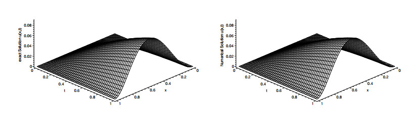
In this study, the so-called generalized differential transform method (GDTM) is developed to derive a semi- analytical solution for fractional partial differential equations which involves Riesz space fractional derivative. We focus primarily on implementing the novel algorithm to fractional telegraph equation with Riesz space-fractional derivative. Some theorems are presented to obtain new algorithm, as well as the error bound is found. This method is dealing with separating the main equation into sub-equations and applying transformation for sub-equations to attain compatible recurrence relations. This process will allow to obtain semi-analytical solution using inverse transformation. To illustrate the reliability and capability of the method, some examples are provided. The results reveal that the algorithm is very effective and uncomplicated.
Citation: S. Mohammadian, Y. Mahmoudi, F. D. Saei. Solution of fractional telegraph equation with Riesz space-fractional derivative[J]. AIMS Mathematics, 2019, 4(6): 1664-1683. doi: 10.3934/math.2019.6.1664
In this study, the so-called generalized differential transform method (GDTM) is developed to derive a semi- analytical solution for fractional partial differential equations which involves Riesz space fractional derivative. We focus primarily on implementing the novel algorithm to fractional telegraph equation with Riesz space-fractional derivative. Some theorems are presented to obtain new algorithm, as well as the error bound is found. This method is dealing with separating the main equation into sub-equations and applying transformation for sub-equations to attain compatible recurrence relations. This process will allow to obtain semi-analytical solution using inverse transformation. To illustrate the reliability and capability of the method, some examples are provided. The results reveal that the algorithm is very effective and uncomplicated.

| [1] | D. Baleanu, J. H. Asad, A. Jajarmi, The fractional model of spring pendulum: new features within different kernels, Proceeding of the Romanian Academy Series A, 19 (2018), 447-454. |
| [2] | M. Hajipour, A. Jajarmi, D. Baleanu, et al. On a accurate discretization of a variable-order fractional reaction-diffusion equation, Commun. Nonlinear Sci., 69 (2019), 119-133. |
| [3] | S. S. Sajjadi, A. Jajarmi, J. H. Asad, New features of the fractional Euler-Lagrange equations for a physical system within non-singular derivative operator, Eur. Phys. J. Plus, 134 (2019), 181. |
| [4] | D. Baleanu, A. Jajarmi, J. H. Asad, Classical and fractional aspects of two coupled pendulums, Rom. Rep. Phys., 71 (2019), 103-115. |
| [5] | S. Kumar, A new analytical modelling for fractional telegraph equation via Laplace transform, Appl. Math. Model., 38 (2014), 3154-3163. |
| [6] | D. Kumar, J. Singh, S. kumar, Analytic and approximate solutions of space-time fractional telegraph equation via Laplace transform, Walailak Journal of Science and Technology (WJST), 11 (2013), 711-728. |
| [7] | Z. Zhao, C. Li, Fractional difference/finite element approximations for time-space fractional telegraph equation, Appl. Math. Comput., 219 (2012), 2975-2988. |
| [8] | Q. Yang, F. liu, I. Turner, Numerical methods for fractional partial differential equations with Riesz space fractional derivatives, Appl. Math. Model., 34 (2010), 200-218. |
| [9] | A. H. Bhrawy, M. Zaky, J. A. Tenreiro Machado, Numerical solution of the two-sided space-time fractional telegraph equation via Chebyshev Tau approximation, J. Optimiz. Theory Appl., 174 (2017), 321-341. |
| [10] | V. R. Hossieni, W. Chen, Z. Avazzadeh, Numerical solution of fractional telegraph equation by using radial basis functions, Eng. Anal. Bound. Elem., 38 (2014), 31-39. |
| [11] | T. Breiten, V. Simoncini, M. Stoll, Low-rank solvers for fractional differential equations, Electron. T. Numer. Anal., 45 (2016), 107-132. |
| [12] | J. K. Zhou, Differential Transformation and Its Application for Electrical Circuits, Wuhan, China: Huazhong University Press, 1986. |
| [13] | C. K. Chen, S. H. Ho, Solving partial differential equations by two-dimensional differential transform method, Appl. Math. Comput., 106 (1999), 171-179. |
| [14] | Z. Odibat, S. Momani, V. S. Erturk, Generalized differential transform method: Application to differential equations of fractional order, Appl. Math. Comput., 197 (2008), 467-477. |
| [15] | Z. Odibat, S. Momani, A generalized differential transform method for linear partial differential equations of fractional order, Appl. Math. Lett., 21 (2008), 194-199. |
| [16] | S. S. Ray, Numerical solution and solitary wave solutions of fractional KDV equations using modified fractional reduced differnatial transform method, Computational Mathematics and Mathematical Physics, 53 (2013), 1870-1881. |
| [17] | E. F. D. Goufo, S. Kumar, Shallow water wave models with and without singular kernel:existenc, uniqueness, and similarities, Math. Probl. Eng., 2017 (2017), 1-9. |
| [18] | B. Soltanalizadeh, differential transform method for solving one-space-dimensional telegraph equation, Comput. Appl. Math., 30 (2011), 639-653. |
| [19] | V. K. Sirvastava, M. K. Awasthi, R. K. Chaurasia, Reduced differential transform method to solve two and three dimensional second order hyperbolic telegraph equations, Journal of King Saud University: Engineering Sciences, 29 (2017), 166-171. |
| [20] | M. Garg, P. Manohar, S. L. Kalla, Generalized differential transform method to space- time fractional telegraph equation, International Journal of Differential equations, 2011 (2011), 1-9. |
| [21] | A. Cetinkaya, O. Kiymaz, The solution of the time-fractional diffusion equation by the generalize differential transform method, Math. Comput. Model., 57 (2013), 2349-2354. |
| [22] | L. Zou, Z. Wang, Z. Zong, Generalized differential transform method to differential-difference equation, Phys. Lett. A, 373 (2009), 4142-4151. |
| [23] | J. Biazar, M. Eslami, Analiytic solution of Telegraph equation by differential transform method, Phys. Lett. A, 374 (2010), 2904-2906. |
| [24] | I. Podlubny, Fractional Differential Equations, SanDiego: Academic Press, 1999. |
| [25] | K. S. Miller, B. Ross, An Introduction to the Fractional Calculus and Fractional Differential Equations, New York: John Wiley & Sons Inc., 1993. |
| [26] | Z. M. Odibat, S. Kumar, N. Shawagfeh, et al. A study on the convergence conditions of generalized differential transform method, Math. Method. Appl. Sci., 40 (2017), 40-48. |
| [27] | S. Chen, X. Jiang, F. Liu, et al. High order unconditionally stable difference schemes for the Riesz space-fractional telegraph equation, J. Comput. Appl. Math., 278 (2015), 119-129. |
| [28] | Y. Zhang, H. Ding, Improved matrix transform method for the Riesz space fractional reaction dispersion equation, J. Comput. Appl. Math., 260 (2014), 266-280. |
| [29] | G. A. Anastassiou, I. K. Argyros, S. Kumar, Monotone convergence of extended iterative methods and fractional calculus with applications, Fund. Inform., 151 (2017), 241-253. |
Figures(2) / Tables(1)

S. Mohammadian, Y. Mahmoudi, F. D. Saei. Solution of fractional telegraph equation with Riesz space-fractional derivative[J]. AIMS Mathematics, 2019, 4(6): 1664-1683. doi: 10.3934/math.2019.6.1664


 DownLoad: