The ability to replace failed spare parts in time directly affects the supportability level of equipment systems. The selection of spare parts' depot locations, inventory mode, and allocation are often separate and independent operations. However, in these situations, the total supply cost is usually relatively high with the consideration of spare parts shortage and maintenance delays. Therefore, this article dealt with a depot location-inventory-allocation problem based on the $ (r, Q) $ inventory method and analyzed a combined network of centralized spare part depot locations, inventory, and allocation. Meanwhile, considering the convenience and speed of spare parts transportation brought about by the improvement of transportation capacity, a network is proposed to adopt a centralized storage and point-to-point allocation strategy for parts replacement, which reduces supportability costs without affecting supply efficiency. An optimization model has been developed that reduces the overall cost of support, including inventory, construction, transportation, and logistics. Three equipment support efficiency metrics were used as constraints in this model to assess the location of open depots: selection availability, fill rate, and predicted downtime. Additionally, due to the knowledge asymmetry, there are some shortage issues which always lead to extra expenditure. The model also introduces uncertain distribution to demand measurement and adopts a genetic algorithm for model solving. Ultimately, a numerical instance was developed so as to verify our results.
Citation: Yaojun Liu, Li Jia, Ping Wang, Xiaolin Song. Joint optimization of location and allocation for spare parts depots under ($ r, Q $) inventory policy[J]. Networks and Heterogeneous Media, 2024, 19(3): 1038-1057. doi: 10.3934/nhm.20240046
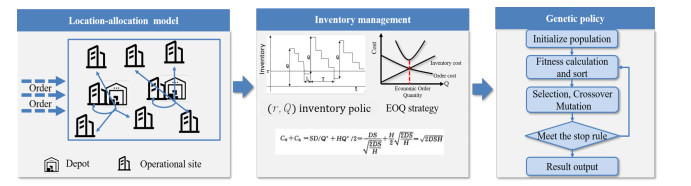
The ability to replace failed spare parts in time directly affects the supportability level of equipment systems. The selection of spare parts' depot locations, inventory mode, and allocation are often separate and independent operations. However, in these situations, the total supply cost is usually relatively high with the consideration of spare parts shortage and maintenance delays. Therefore, this article dealt with a depot location-inventory-allocation problem based on the $ (r, Q) $ inventory method and analyzed a combined network of centralized spare part depot locations, inventory, and allocation. Meanwhile, considering the convenience and speed of spare parts transportation brought about by the improvement of transportation capacity, a network is proposed to adopt a centralized storage and point-to-point allocation strategy for parts replacement, which reduces supportability costs without affecting supply efficiency. An optimization model has been developed that reduces the overall cost of support, including inventory, construction, transportation, and logistics. Three equipment support efficiency metrics were used as constraints in this model to assess the location of open depots: selection availability, fill rate, and predicted downtime. Additionally, due to the knowledge asymmetry, there are some shortage issues which always lead to extra expenditure. The model also introduces uncertain distribution to demand measurement and adopts a genetic algorithm for model solving. Ultimately, a numerical instance was developed so as to verify our results.

| [1] |
J. Wu, H. Liu, H. Zuo, Y. Yang, Y. Ma, L. Kong, The demand supply steady-state process-based multi-level spare parts optimization, Sensors, 21 (2021), 8324. https://doi.org/10.3390/s21248324 doi: 10.3390/s21248324

|
| [2] | G. J. Van Houtum, B. Kranenburg, Spare Parts Inventory Control under System Availability Constraints, 227 (2015), Springer: Berlin. |
| [3] | Z. Jia, Z. Zeng, Y. Zhou, Y. Zhou, Configuration optimization methods for multi-echelon and multi-constraints spare parts based on dynamic demands, in 2014 10th International Conference on Reliability, Maintainability and Safety (ICRMS), (2014), 1091–1096. https://doi.org/10.1109/ICRMS.2014.7107372 |
| [4] |
J. Holmström, J. Partanen, J. Tuomi, M. Walter, Rapid manufacturing in the spare parts supply chain: Alternative approaches to capacity deployment, J. Manuf. Technol. Manage., 21 (2010), 687–697. https://doi.org/10.1108/17410381011063996 doi: 10.1108/17410381011063996
|
| [5] |
W. D. Rustenburg, G. J. van Houtum, W. H. M. Zijm, Spare parts management for technical systems: Resupply of spare parts under limited budgets, IIE trans., 32 (2000), 1013–1026. https://doi.org/10.1023/A:1007676901673 doi: 10.1023/A:1007676901673
|
| [6] |
A. Diaz, M. C. Fu, Models for multi-echelon repairable item inventory systems with limited repair capacity, Eur. J. Oper. Res., 97 (1997), 480–492. https://doi.org/10.1016/S0377-2217(96)00279-2 doi: 10.1016/S0377-2217(96)00279-2
|
| [7] |
S. Van der Auweraer, R. Boute, Forecasting spare part demand using service maintenance information, Int. J. Prod. Econ., 213 (2019), 138–149. https://doi.org/10.1016/j.ijpe.2019.03.015 doi: 10.1016/j.ijpe.2019.03.015
|
| [8] |
E. F. Israel, A. Albrecht, E. M. Frazzon, B. Hellingrath, Operational supply chain planning method for integrating spare parts supply chains and intelligent maintenance systems, IFAC-PapersOnLine, 50 (2017), 12428–12433. https://doi.org/10.1016/j.ifacol.2017.08.2432 doi: 10.1016/j.ifacol.2017.08.2432
|
| [9] | S. Gupta, Working capital management through inventory management techniques, Ashok Yakkaldevi, 2020. |
| [10] |
W. J. Kennedy, J. W. Patterson, L. D. Fredendall, An overview of recent literature on spare parts
inventories, Int. J. Prod. Econ., 76 (2002), 201–215. https://doi.org/10.1016/S0925-5273(01)00174-8 doi: 10.1016/S0925-5273(01)00174-8
|
| [11] |
M. Wen, Q. Han, Y. Yang, R. Kang, Uncertain optimization model for multi-echelon spare parts supply system, Appl. Soft Comput., 56 (2017), 646–654. https://doi.org/10.1016/j.asoc.2016.07.057 doi: 10.1016/j.asoc.2016.07.057
|
| [12] |
L. Turrini, J. Meissner, Spare parts inventory management: New evidence from distribution fitting, Eur. J. Oper. Res., 273 (2019), 118–130. https://doi.org/10.1016/j.ejor.2017.09.039 doi: 10.1016/j.ejor.2017.09.039
|
| [13] |
A. Van Horenbeek, J. Buré, D. Cattrysse, L. Pintelon, P. Vansteenwegen, Joint maintenance and inventory optimization systems: A review, Int. J. Prod. Econ., 143 (2013), 499–508. https://doi.org/10.1016/j.ijpe.2012.04.001 doi: 10.1016/j.ijpe.2012.04.001
|
| [14] | G. Laporte, S. Nickel, F. Saldanha-da-Gama, Introduction to Iocation Science, Springer International Publishing, (2019), 1–21. |
| [15] |
R. Z. Farahani, M. Hekmatfar, B. Fahimnia, N. Kazemzadeh, Hierarchical facility location problem: Models, classifications, techniques, and applications, Comput. Ind. Eng., 68 (2014), 104–117. https://doi.org/10.1016/j.cie.2013.12.005 doi: 10.1016/j.cie.2013.12.005
|
| [16] |
S. Kheybari, M. Kazemi, J. Rezaei, Bioethanol facility location selection using best-worst method, Appl. Energy, 242 (2019), 612–623. https://doi.org/10.1016/j.apenergy.2019.03.054 doi: 10.1016/j.apenergy.2019.03.054
|
| [17] |
T. Uslu, O. Kaya, Location and capacity decisions for electric bus charging stations considering waiting times, Transp. Res. Part D Transp. Environ., 90 (2021), 102645. https://doi.org/10.1016/j.trd.2020.102645 doi: 10.1016/j.trd.2020.102645
|
| [18] |
E. Gebennini, R. Gamberini, R. Manzini, An integrated production–distribution model for the dynamic location and allocation problem with safety stock optimization, Int. J. Prod. Econ., 122 (2009), 286–304. https://doi.org/10.1016/j.ijpe.2009.06.027 doi: 10.1016/j.ijpe.2009.06.027
|
| [19] |
D. R. Fernandes, C. Rocha, D. Aloise, G. M. Ribeiro, E. M. Santos, A. Silva, A simple and effective genetic algorithm for the two-stage capacitated facility location problem, Comput. Ind. Eng., 75 (2014), 200–208. https://doi.org/10.1016/j.cie.2014.05.023 doi: 10.1016/j.cie.2014.05.023
|
| [20] | R. Rahmaniani, M. Saidi-Mehrabad, H. Ashouri, Robust capacitated facility location problem optimization model and solution algorithms, J. Uncertain Syst., 7 (2023), 22–35. |
| [21] |
B. Hamdan, A. Diabat, A two-stage multi-echelon stochastic blood supply chain problem, Comput. Oper. Res., 101 (2019), 130–143. https://doi.org/10.1016/j.cor.2018.09.001 doi: 10.1016/j.cor.2018.09.001
|
| [22] |
W. Wu, W. Zhou, Y. Lin, Y. Xie, W. Jin, A hybrid metaheuristic algorithm for location inventory routing problem with time windows and fuel consumption, Expert Syst. Appl., 166 (2021), 114034. https://doi.org/10.1016/j.eswa.2020.114034 doi: 10.1016/j.eswa.2020.114034
|
| [23] |
Z. Dai, F. Aqlan, X. Zheng, K. Gao, A location-inventory supply chain network model using two heuristic algorithms for perishable products with fuzzy constraints, Comput. Ind. Eng., 119 (2018), 338–352. https://doi.org/10.1016/j.cie.2018.04.007 doi: 10.1016/j.cie.2018.04.007
|
| [24] |
H. Y. Mak, Z. J. Shen, Risk diversification and risk pooling in supply chain design, IIE Trans., 44 (2012), 603–621. https://doi.org/10.1080/0740817X.2011.635178 doi: 10.1080/0740817X.2011.635178
|
| [25] | E. Topan, Z. P. Bayındır, T. Tan, An exact solution procedure for multi-item two-echelon spare parts inventory control problem with batch ordering in the central depot, Oper. Res. Lett., 38 (2010), 454–461. |
| [26] | D. Ozdemir, Collaborative Planning and Replenishment Policies, INSEAD (France and Singapore), 2004. |
| [27] |
R. J. Basten, R. J. Schutten, M. C. Van Der Heijden, An efficient model formulation for level of repair analysis, Ann. Oper. Res., 172 (2009), 119–142. https://doi.org/10.1007/s10479-009-0516-5 doi: 10.1007/s10479-009-0516-5
|
| [28] |
R. J. Basten, M. C. Van der Heijden, J. M. Schutten, Joint optimization of level of repair analysis and spare parts stocks, Eur. J. Oper. Res., 222 (2012), 474–483. https://doi.org/10.1016/j.ejor.2012.05.045 doi: 10.1016/j.ejor.2012.05.045
|
| [29] |
N. Gülpınar, D. Pachamanova, E. Çanakoğlu, Robust strategies for facility location under uncertainty, Eur. J. Oper. Res., 225 (2013), 21–35. https://doi.org/10.1016/j.ejor.2012.08.004 doi: 10.1016/j.ejor.2012.08.004
|
| [30] |
E. Saha, P. K. Ray, Modelling and analysis of inventory management systems in healthcare: A review and reflections, Comput. Ind. Eng., 137 (2019), 106051. https://doi.org/10.1016/j.cie.2019.106051 doi: 10.1016/j.cie.2019.106051
|
| [31] |
S. Küçükyavuz, R. Jiang, Chance-constrained optimization under limited distributional information: A review of reformulations based on sampling and distributional robustness, EURO J. Comput. Optim., 10 (2022), 100030. https://doi.org/10.1016/j.ejco.2022.100030 doi: 10.1016/j.ejco.2022.100030
|
| [32] | J. Long, R. Kang, H. L. Cheng, Optimization of spares supply based on integrated supply performance measure, Syst. Eng. Electron., 29 (2007), 2085–2087. |
| [33] | S. P. Sarmah, U. C. Moharana, Spare parts inventory management literature and direction towards the use of data mining technique: A review, Handb. Res. Promoting Bus. Process Improv. Through Inventory Control Tech., 2018,534–558. https://doi.org/10.4018/978-1-5225-3232-3.ch028 |
| [34] |
B. K. Lad, M. S. Kulkarni, Integrated reliability and optimal maintenance schedule design: A life cycle cost based approach, Inter. J. Prod. Lifecycle Manage., 3 (2008), 78–90. https://doi.org/10.1504/IJPLM.2008.019971 doi: 10.1504/IJPLM.2008.019971
|
| [35] |
W. Wu, J. Ma, R. Liu, W. Jin, Multi-class hazmat distribution network design with inventory and superimposed risks, Transp. Res. Part E Logist. Transp. Rev., 161 (2022), 102693. https://doi.org/10.1016/j.tre.2022.102693 doi: 10.1016/j.tre.2022.102693
|
| [36] |
W. Wu, Y. Li, Pareto truck fleet sizing for bike relocation with stochastic demand: Risk-averse multi-stage approximate stochastic programming, Transp. Res. Part E Logist. Transp. Rev., 183 (2024), 103418. https://doi.org/10.1016/j.tre.2024.103418 doi: 10.1016/j.tre.2024.103418
|
| [37] |
P. Li, M. Wen, T. Zu, R. Kang, A joint location–allocation–inventory spare part optimization model for base-level support system with uncertain demands, Axioms, 12 (2023), 46. https://doi.org/10.3390/axioms12010046 doi: 10.3390/axioms12010046
|
| [38] |
A. De, S. P. Singh, Analysis of fuzzy applications in the agri-supply chain: A literature review, J. Cleaner Prod., 283 (2021), 124577. https://doi.org/10.1016/j.jclepro.2020.124577 doi: 10.1016/j.jclepro.2020.124577
|
| [39] | B. Liu, Uncertainty Theory, Springer Berlin Heidelberg, (2010), 1–79. |


Figures(5) / Tables(4)
Yaojun Liu, Li Jia, Ping Wang, Xiaolin Song. Joint optimization of location and allocation for spare parts depots under ($ r, Q $) inventory policy[J]. Networks and Heterogeneous Media, 2024, 19(3): 1038-1057. doi: 10.3934/nhm.20240046


 DownLoad: