This paper is devoted to the study of the bitemperature Euler system in a polyatomic setting. Physically, this model describes a mixture of one species of ions and one species of electrons in the quasi-neutral regime. We firstly derive the model starting from a kinetic polyatomic model and performing next a fluid limit. This kinetic model is shown to satisfy fundamental properties. Some exact solutions are presented. Finally, a numerical scheme is derived and proved to coincide with an approximation designed in [
Citation: Denise Aregba-Driollet, Stéphane Brull. Modelling and numerical study of the polyatomic bitemperature Euler system[J]. Networks and Heterogeneous Media, 2022, 17(4): 593-611. doi: 10.3934/nhm.2022018
This paper is devoted to the study of the bitemperature Euler system in a polyatomic setting. Physically, this model describes a mixture of one species of ions and one species of electrons in the quasi-neutral regime. We firstly derive the model starting from a kinetic polyatomic model and performing next a fluid limit. This kinetic model is shown to satisfy fundamental properties. Some exact solutions are presented. Finally, a numerical scheme is derived and proved to coincide with an approximation designed in [

| [1] |
A comment on the computation of non-conservative products. J. Comput. Phys. (2010) 229: 2759-2763. 
|
| [2] |
Entropy condition for the ES BGK model of Boltzmann equation for mono and polyatomic gases. Eur. J. Mech. B Fluids (2000) 19: 813-830.
|
| [3] |
Modelling and numerical approximation for the nonconservative bitemperature Euler model. ESAIM Math. Model. Numer. Anal. (2018) 52: 1353-1383.
|
| [4] |
A viscous approximation of the bitemperature Euler system. Comm. Math. Sci. (2019) 17: 1135-1147.
|
| [5] |
Global existence of smooth solutions for a non-conservative bitemperature Euler model. SIAM J. Math. Anal. (2021) 53: 1886-1907.
|
| [6] |
A discrete velocity numerical scheme for the two-dimensional bitemperature Euler system. SIAM J. Numer. Anal. (2022) 60: 28-51.
|
| [7] |
Discrete kinetic schemes for multidimensional systems of conservation laws. SIAM J. Numer. Anal. (2000) 37: 1973-2004.
|
| [8] |
Monoatomic rarefied gas as a singular limit of polyatomic gas in extended thermodynamics. Physics letter A (2013) 337: 2136-2140.
|
| [9] |
On the Chapman-Enskog asymptotics of mixture of monoatomic and polyatomic rarefied gases. Kin. Rel. Mod. (2018) 11: 821-858.
|
| [10] |
BGK polyatomic model for rarefied flows. J. Sci. Comput. (2019) 78: 1893-1916.
|
| [11] |
M. Bisi, R. Monaco and A. J. Soares, A BGK model for reactive mixtures of polyatomic gases with continuous internal energy, J. Phys. A, 51 (2018), 125501, 29 pp. |
| [12] |
Dynamical pressure in a polyatomic gas: Interplay between kinetic theory and Extended Thermodynamics. Kinet. Relat. Models (2018) 11: 71-95.
|
| [13] |
On a kinetic BGK model for slow chemical reactions. Kinet. Relat. Models (2011) 4: 153-167.
|
| [14] |
M. Bisi and R. Travaglini, A polyatomic model for mixtures for monoatomic and polyatomic gases, Phys. A, 547 (2020), 124441, 18 pp. |
| [15] |
A general consistent BGK model for gas mixtures. Kinet. Relat. Models (2018) 11: 1377-1393.
|
| [16] |
Statistical collision model for Monte-Carlo simulation of polyatomic mixtures. Journ. Comput. Phys. (1975) 18: 405-420.
|
| [17] | Microreversible collisions for polyatomic gases and Boltzmann's theorem. Eur. Journ. Fluid Mech. (1994) 13: 237-254. |
| [18] | (2000) Hyperbolic Systems of Conservation Laws. Oxford: Oxford Lecture Series in Mathematics and its Applications, 20. Oxford University Press. |
| [19] |
An Ellipsoidal Statistical Model for a monoatomic and polyatomic gas mixture. Comm. Math. Sci. (2021) 19: 2177-2194.
|
| [20] |
A kinetic approach of the bi-temperature Euler model. Kinet. Relat. Models (2020) 13: 33-61.
|
| [21] |
On the Ellipsoidal Statistical Model for polyatomic gases. Cont. Mech. Thermodyn (2009) 20: 489-508.
|
| [22] |
Navier-Stokes equations with several independent pressure laws and explicit predictor-corrector schemes. Numer. Math. (2005) 101: 451-478.
|
| [23] |
Numerical methods for weakly ionized gas. Astrophysics and Space Science (1998) 260: 15-27.
|
| [24] | Definition and weak stability of nonconservative products. J. Math. Pures et Appl. (1995) 74: 483-548. |
| [25] |
Sur un modèle de type Borgnakke-Larsen conduisant à des lois d'énergie non-linéaires en température pour les gas parfaits polyatomiques. Ann. Fac. Sci. Toulouse Math. (1997) 6: 257-262.
|
| [26] |
A kinetic model allowing to obtain the energy law of polytropic gases in the presence of chemical reactions. Eur. J. Mech. B Fluids (2005) 24: 219-236.
|
| [27] | The kinetic equilibrium regime. Physica A (1998) 260: 49-72. |
| [28] |
E. Estibals, H. Guillard and A. Sangam, Derivation and numerical approximation of two-temperature Euler plasma model, J. Comput. Phys., 444 (2021), 110565, 48 pp. |
| [29] | Poiseuille flow and thermal transpiration of a rarefied polyatomic gas through a circular tube with applications to microflows. Boll. Unione Mat. Ital. (2011) 4: 19-46. |
| [30] |
V. Giovangigli, Multicomponent Flow Modeling. Modeling and Simulation in Science, Engineering and Technology, Birkhäuser Boston, Inc., Boston, MA, 1999. |
| [31] |
Kinetic theory of plasmas. Maths models and methods in the Appl. Sci. (2009) 19: 527-599.
|
| [32] | Improved Bhatnagar-Gross-Krook model of electron-ion collisions. Phys.Fluids (1973) 16: 2022-2023. |
| [33] |
J. D. Huba, NRL Plasma Formulary, Revised 2013 version, NRL. |
| [34] |
A consistent kinetic model for a two-component mixture of polyatomic molecules. Comm. in Math. Sci. (2019) 17: 149-173.
|
| [35] |
Shock wave structure in polyatomic gases: Numerical analysis using a model Boltzmann equation. AIP Conf. Proc. (2016) 1786: 180004.
|
| [36] |
Numerical methods for nonconservative hyperbolic systems: A theoretical framework. SIAM J. Numer. Anal. (2006) 44: 300-321.
|
| [37] |
A kinetic scheme for the Saint-Venant system with a source term. Calcolo (2001) 38: 201-231.
|
| [38] |
Fluid modeling for the Knudsen compressor: Case of polyatomic gases. Kinet. Relat. Models (2010) 3: 353-372.
|
| [39] |
Q. Wargnier, S. Faure, S. B. Graille, T. Magin and M. Massot, Numerical treatment of the nonconservative product in a multiscale fluid model for plasmas in thermal nonequilibrium: Application to solar physics, SIAM J. Sci. Comput., 42 (2020), B492–B519. |
| [40] | (1966) Physics of Shock Waves and High-Temperature Hydrodynamic Phenomena. Academic Press. |
Figures(5)
Denise Aregba-Driollet, Stéphane Brull. Modelling and numerical study of the polyatomic bitemperature Euler system[J]. Networks and Heterogeneous Media, 2022, 17(4): 593-611. doi: 10.3934/nhm.2022018

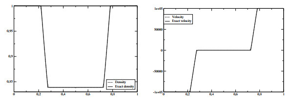
Double rarefaction. Left: density. Right: velocity
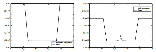
Double rarefaction. Left: electronic temperature. Right : ionic temperature
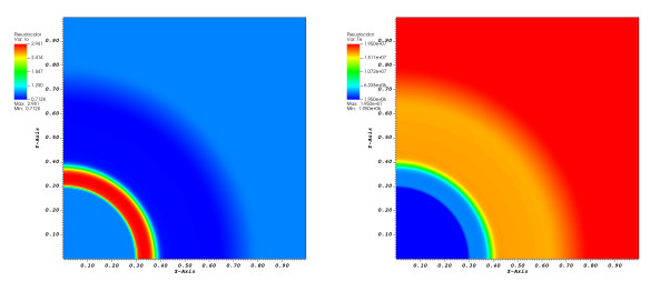
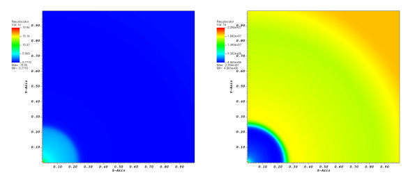
Total density (left) and electronic temperature (right) at time
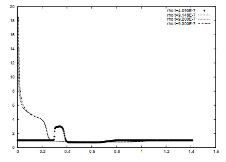
Implosion test case with
Implosion test case with


 DownLoad: