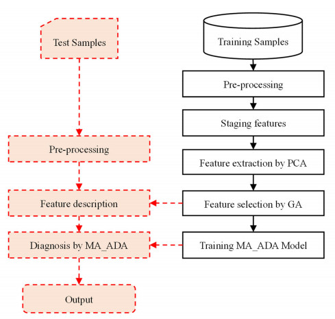
Cardiovascular disease classification based on a multi-classification integrated model

1.   Introduction

Today, cardiovascular disease (CVD) has become the leading cause of death in the world. In the meantime, coronary artery disease (CAD) is the most common type of CVD, whose diagnosis in the early stages can save people's lives. However, finding and analyzing the disease symptoms in its initial stages is not an easy task. Usually, accurate diagnosis of the disease is a time-consuming, expensive, and error-prone process. If CVD is not detected in its early stages, the patient may face bad consequences and life-threatening situations, which makes handling their condition more challenging. These conditions make the lack of timely diagnosis of CVD, in addition to threatening the patient's life, put double pressure on their condition and the medical system; and at the same time, it also aggravates the tension of medical resource allocation ^[1,2].

The occurrence of CVD is affected by a variety of risk factors. These factors are related to attributes such as basic information about the patient, the patient's blood routine, heart ultrasound, and biochemical examination of the patients; and the risk of CVD can be predicted and regulated by controlling these risk factors ^[3]. So in real life, we can, through the observation of the risk factors associated with CVD in patients, predict whether CVD happens in them, and according to these CVD risk factors, the possibility of disease in people can be minimized. At the same time, the prediction of CVD needs to be accurate and fast, so as to ensure the timely treatment, prevention and control of CVD, and to cope with various emergencies ^[4]. Therefore, an important problem in the prediction of CVD is how to make effective use of the disease information provided by patients to achieve rapid and effective prediction of CVD ^[5,6]. Today, machine learning techniques are widely used in disease diagnosis applications, and CVD diagnosis has been one of the topics of researchers' attention in recent years due to its importance. But despite the many kinds of research done on this issue, there are still challenges that motivate the current research. Relatively low accuracy is one of the limitations of classical machine learning techniques. Whereas it seems that this problem can be solved to some extent by using combined classifiers on the other hand, a CVD diagnosis system should be able to predict the disease based on different information so that the diagnosis process can still be performed with acceptable accuracy in the presence of incomplete clinical information or lack of access to some tests.

This paper will make effective use of the patient's condition information through scientific and effective methods, identify the risk factors of CVD and predict CVD according to these risk factors in order to guide the treatment and life of patients according to these factors, effectively reduce the probability of disease of patients, ensure that patients can carry out timely treatment, improve the physical health of patients, reduce the medical burden of patients and society and optimize the allocation of social medical resources. The contribution of this paper is twofold:

1. This research conducts a four-stage multi-classification study on the prediction of coronary heart disease. In this regard, a set of 54 features is divided into four cumulative groups based on their acquisition period, and a set of top N features is used for prediction. This scheme can be effective in determining the most relevant features of the existence of CVD in patients.

2. In this research, a new architecture of the Adaboost classifier, named Multi-Agent Adaboost (MA_ADA) has been proposed to diagnose CVD. This classifier model includes a set of Adaboost classifiers, each of which is formed separately by a different subset of database instances and weighted according to its training performance. Also, the multi-agent principle is used to produce the output of MA_ADA for test instances.

The remainder of this paper is organized as follows: Section 2 contains the literature review. In Section 3, the research method is described in detail, and in Section 4, implementation results are discussed. In Section 5, conclusions have been made and several suggestions are provided for continuing this research path.

2.   Literature review

CVD has become the world's highest mortality rate of chronic diseases at present and brought a heavy burden of medical resources to various countries. At the same time, it seriously influences the patient's life, reduces the patient's quality of life and fast effective projections for CVD will be able to help patients and doctors find patients with CVD risk as soon as possible. In this way, patients can be provided with effective treatment, avoid the deterioration of the disease and reduce the burden of disease on patients and the medical system.

The prediction of CVD is usually based on the associated risk factors, and the way in which information on these risk factors is obtained varies. Some risk factors can be obtained by doctors' direct inquiry or simple examination, while some risk factors need to be obtained through complex medical examination, which will consume a lot of time and have certain requirements on medical conditions. Therefore, it takes a lot of time to obtain complete information about the patient's condition, and assessing the patient's condition will be delayed. A lot of scholars have pointed out the importance of fast and accurate prediction, such as Gregor ^[7], who pointed out that making a rapid accurate diagnosis for the disease forecast has a vital significance, will help the patient's condition for effective management and control and make the patient get timely and effective treatment. Uguroglu et al. ^[8] tried to predict Coronary Heart Disease (CHD) in patients by using the most convenient and fast information of risk factors, so as to achieve the risk stratification of CHD in patients and provide guidance for the follow-up treatment of patients. However, the above kinds of literature that emphasized the need for rapid prediction of CVDs did not put forward a feasible criterion to guide the rapid and accurate prediction of CVDs, and the selection of risk factors for rapid prediction was highly subjective and fuzzy. The different ways of gaining information about CVD risk factors, and the time needed to obtain this information, cause some limitations on the ability of this method for accurate and quick predictions of CVD in patients. Because, some risk factors require a longer time to be acquired. Therefore, considering time required to obtain information on each risk factor is important. Kukar et al. ^[9] proposed that the characteristics of the information be divided into several different categories according to the cost of access to information and how fast the information of risk factors can be obtained. The authors examined CVD diagnosis with a variety of machine learning methods. Different combinations of risk factors were evaluated, so the effect of each risk factor on CVD prediction accuracy was examined. This article, motivated the idea of our study, which categorize different risk factors of CVD according to time spent for obtaining their information and attempting to determine the risk factors which can lead to an accurate CVD diagnosis model with least required time to obtain patient information.

At present, research on CVD prediction can be mainly divided into two categories, one is the traditional research on CVD prediction, and the other is about the application of new machine learning methods in CVD prediction. Traditional studies on the prediction of CVDs are mainly about the establishment of CVD risk assessment models. Such studies mainly collect massive follow-up data from a large number of patients for long-term follow-up and build risk assessment models based on these follow-up data according to risk factors.

For CVD, a series of risk assessment models have been developed at home and abroad. Among these models, the Framingham risk assessment model in the United States is the earliest one. This risk assessment model was organized by the US government in the 1940s to carry out CVD-related research by relevant medical staff on the basis that CVD had become the leading cause of death in the American population ^[10]. Researchers conducted long-term studies and follow-ups on a large number of people and proposed the concept of risk factors, thus laying a basic model for the subsequent establishment of CVD risk assessment models. Researchers constructed CVD risk assessment models based on risk factors using the logistic multiple regression method. To evaluate the patient's risk of CVD in 10 years, this model included multiple CVD events as the endpoint time, such as CVD and stroke ^[11,12,13]. The Framingham model is of pioneering significance for the prediction of CVD, and a large number of CVD risk assessment models have been established on the basis of the Framingham model since then.

Since the Framingham model was mainly targeted at white Americans when it was established, its prediction effect in other groups was not good ^[14,15,16]. Therefore, it can be seen that Framingham's risk assessment model cannot be perfectly applied to all groups. Countries are developing CVD risk assessment models suitable for their populations.

In view of the serious situation of the development of CVDs around the world, in 2008, the World Health Organization (WHO) issued a pocket guide for CVD risk assessment and management, aiming at the prevention and control of CVDs ^[17]. The guidelines are intended to provide advice on CVD prevention and control for potential patients with CVD and to provide WHO/ International Society of Hypertension (ISH) CVD risk projections, which are only valid for prediction in the WHO subregion of middle and high-income countries in the Western Pacific.

For prediction models of CVD in general, the method used by most is based on the traditional method of survival analysis, mainly for the analysis of logistic regression and Cox proportional hazards on the risk factors in the selection of certain subjective factors. At the same time, due to differences in study population, the risk assessment model can't apply to all people. With the passing of time, the research population based on the prediction model is different from today's population, and the original evaluation system is not necessarily suitable for today's population. With the development of science and technology and the acceleration of information exchange, modern popular machine learning methods provide another brand new possibility for CVD risk analysis.

The machine learning method is a scientific computing method based on the rapid development of modern computers and information technology. Relying on its powerful computing power, any problem that can be abstracted into machine learning can be solved by using the machine learning method.

2.1.   CVD diagnosis using machine learning techniques

In the medical field, traditional disease prediction relies on doctors' personal experience and expensive examinations, which are prone to errors and increase medical costs for patients and society. Machine learning methods rely on their powerful ability to learn. Data are being gradually applied to the field of medical information with machine learning methods, to predict the patient's illness based on the patient's data. This prediction can assist the doctor in medical decision making and reduce the medical burden of patients, compared with traditional statistical analysis methods. At present, a large number of domestic and foreign scholars have applied machine learning methods to the prediction of CVDs.

At present, many machine learning methods have been applied to the prediction of CVDs, among which, K-nearest neighbor classifier, support vector machine, neural network and other algorithms have been widely used. Weng et al. ^[18] evaluated whether machine learning could improve the prediction of cardiovascular risk based on prospective cohort studies and concluded that the machine learning algorithm could significantly improve the prediction effect of cerebrovascular disease risk, indicating the effectiveness and feasibility of the machine learning method in the prediction of CVD. Gilani et al. ^[19] used a K-nearest-neighbor classifier to classify electrocardiogram (ECG) signals and predict atrial fibrillation, and the results showed that the K-nearest-neighbor classifier achieved 98% sensitivity and 95% specificity, showing good applicability in the prediction of ECG signals. In addition, researchers also combined the K-neighbor classifier with other methods for prediction. Porta et al. ^[20] combined a K-nearest neighbor classifier with conditional entropy to control and analyze the complexity of short-term CVDs, while Polat et al. ^[21] combined a K-nearest neighbor classifier with an artificial immune recognition system. Heart disease was diagnosed and validated using data from the University of California, Irvine (UCI) dataset, resulting in 87% accuracy. Support vector machines and neural networks are also widely used in the prediction of CVDs. Patidar et al. ^[22] applied least-squares support vector machines to the analysis of ECG signals and predicted the occurrence of CVDs by improving the kernel function of support vector machines. Amin et al. ^[23] made use of the neural network to diagnose and predict heart disease based on related risk factors and optimized and adjusted the weight in the Genetic Algorithm (GA) degree neural network, finally achieving a prediction accuracy of 89%. Alizadehsani et al. ^[24] applied the Bagging algorithm, Sequential Minimal Optimization (SMO), Naive Bayes and decision tree algorithm to the classification and prediction of CVDs, and found that SMO and Bagging algorithm achieved the best classification effect with an accuracy of 89%. Hijazi et al. ^[25] applied the K-nearest neighbor algorithm, support vector machine, random forest and integrated learning algorithm to the ECG data processing of patients with a large amount of data generated by portable devices to predict the risk of CVD and achieved good results. Acharya et al. ^[26] used a convolutional neural network to predict myocardial infarction according to electrocardiogram signals, achieving an accuracy of 93.53% and 95.22%, respectively, in the case of noise and no noise elimination. Fuster-Parra et al. ^[27] applied a Bayesian network to build a CVD risk prediction model. To analyze the relationship between different risk factors and their impact on the risk of developing or dying from CVD, so as to prevent and control CVD.

In the prediction of CVD, because of the characteristics of the clinical data, usually the characteristics of high dimensional data of CVD, the medical data usually contains a large number of features. In the process of disease prediction, however, too much information will affect the performance of the model. Therefore, in the process of classification prediction, we need the raw data for dimension reduction. Key features conducive to prediction were screened out and irrelevant and redundant features were eliminated so as to identify the risk factors that have a key impact on the occurrence of the disease. At present, there is a lot of research combining the dimensionality reduction method with the classification prediction model to obtain a better prediction effect.

In current studies, dimensionality reduction of high-dimensional data can be mainly divided into two types. One is feature extraction, that is, combining original features to form new mutually independent features. At present, this dimensionality reduction method is mainly based on principal component analysis. Giri et al. ^[28] applied linear discriminant analysis (LDA) and independent principal component analysis (ICA) to the feature screening of ECG signal data, and the methods of support vector machine, probabilistic neural network and K-nearest neighbor classification are used to process the data after dimensionality reduction. Good results are achieved. Davari et al. ^[29] applied principal component analysis to ECG signal analysis, extracted heart rate variability signal and applied support vector machine method for diagnosis, reaching 99.2% accuracy. This study shows that the method based on biological signal feature extraction is conducive to improving the accuracy of patient health prediction.

Dimension reduction methods in the literature use the characteristics of the original information to form a new set of features. But in the actual clinical application, it is preferred to reduce the dimensionality of data without changing the original feature information. This operation is usually done on the basis of final prediction results or relevance of attributes; and has formed the second kind of dimension reduction approaches namely feature selection. The feature selection algorithm of filter form, which separates feature selection from the classification prediction model, has been widely used in feature selection of CVDs. Dominic et al. ^[30] conducted feature screening on heart disease data containing 13 features and 75 features in the UCI dataset, respectively, based on the genetic algorithm and information gain method. Naive Bayes, decision trees, support vector machines, linear regression, multilayer perceptron and integrated learning algorithms were used to classify the heart disease data after feature screening. It was found that the effect of feature screening on the heart disease data containing 75 features was better than that on the heart disease data containing 13 features, indicating that feature screening on the data containing a large number of features is necessary to extract key information. Kukar et al. ^[4] diagnosed and predicted ischemic heart disease by analyzing electrocardiogram signals, applied information gain, relied-F and Chi-square test to screen features, and analyzed data by Back Propagation (BP) neural network, naive Bayes, decision tree and K-nearest Neighbor algorithm. By observing the expression of the Receiver Operating Characteristic (ROC) curve to evaluate the effect of prediction classification, it is found that the classification algorithm can achieve better results on the data after feature screening. Verma et al. ^[31] used the combination of particle swarm optimization and K-means clustering to identify risk factors in feature subsets selected according to correlation features and used supervised learning methods such as multi-layer perceptron, multiple Logistic regression, fuzzy disordered rule induction algorithm and C4.5 to predict CVDs. The final results show that the multilayer perceptron has a higher classification accuracy of 88.4%.

At the same time, the feature selection method in wrapper form by combining the classifier with the corresponding feature search algorithm is also widely used in the prediction of CVDs. At present, support vector machine (SVM) is the most widely used low-level classifier in wrapper-form feature selection algorithms. Shilaskar et al. ^[32] proposed a feature selection method based on SVM forward selection, applied it to the diagnosis and prediction of CVDs, and conducted experiments on multiple data sets. The results show that compared with other feature selection methods such as backward elimination and forward inclusion, the proposed method can obtain maximum accuracy. At the same time, Tania et al. ^[33] applied the method of support vector machine combined with backward recursive elimination to the analysis of arterial pulse waveform, and proposed the key waveform signal features, achieving an accuracy of 95.2%.

Ozcift et al. ^[34] used the method of random forests to feature selection for cancer data, and by using 15 kinds of widely used classifiers, such as support vector machine (SVM) and naive Bayesian classifier, results show that the classifier in a random forest performs better. Hu et al. ^[35] applied the random forest feature selection method to the selection of important symptoms of five endogenous pathogens and established evaluation criteria for feature selection through the random forest. The results showed that the method was a high-performance diagnostic model.

Shah et al. ^[36] used a combination of feature selection and feature extraction algorithms for diagnosing CVD. In their work, they used two feature selection mechanisms, including the Mean Fisher-based feature selection algorithm (MFFSA) and the accuracy-based feature selection algorithm (AFSA). Then, the results of these two algorithms were further reduced by PCA. Finally, an SVM model was used to predict CVD. Burse et al. ^[37] researched the effect of various preprocessing techniques on the prediction accuracy of Artificial Neural Networks (ANNs) for CVD diagnosis. Their ANN is a multi-layer pi-sigma neuron model (MLPSNM), which uses a bi-planar sigmoid as its activation function and back-propagation as the training algorithm. This model is fed with normalized, PCA, and linear discriminant analysis (LDA) features for CVD diagnosis.

Repaka et al. ^[38] introduced a Naïve Bayes model for predicting CVD. They have implemented their method on a mobile framework to be used in real-world applications. Reza et al. ^[39], made an attempt to improve the accuracy of CVD prediction by majority voting mechanism of ensemble learning systems. Their ensemble model consists of logistic regression, multi-layer perceptron and Naïve Bayes classifiers. The voting mechanism is effective in improving prediction accuracy compared to individual learners. Velusamy and Ramasamy ^[40] proposed a heterogeneous ensemble model for predicting CVD. Their model includes SVM, Random Forest (RF) and K-nearest neighbor algorithms. They also used RF and SVM for feature selection and determining the feature importance, respectively. This research utilized majority voting, average voting and weighted average voting for CVD prediction, where the last two mechanisms outperform the first one.

Li et al. ^[41] focused on diagnosing CVD by analyzing ECG and phonocardiogram (PCG) signals and proposed a novel multi-modal machine learning-based model for this task. In their research, they used a Convolutional Neural Network (CNN) to encode features of ECG and PCG signals. Then, GA was used to select the most relevant feature set. Finally, the selected features were classified by an SVM model. The multi-modal strategy has proved to be superior to single-modal methods and other alternative methods.

Despite the abundant research conducted in the field of CVD diagnosis using machine learning techniques, there are still some gaps in this research area. The functionality of the model with incomplete patient information is one of the main issues targeted in this research.

3.   Research method

Diagnosing CVD is a challenging task because various attributes may be effective in designing an accurate diagnosis system. Choosing the right set of features in addition to using an efficient classifier are among the most effective factors. In this section, the proposed method for diagnosing CVD is described in detail. The proposed method includes four main steps:

1. Pre-processing and stage-wise grouping of features;

2. Feature extraction by PCA;

3. Feature selection/reduction by GA;

4. classification by MA_ADA.

These steps are illustrated in a diagram in Figure 1.

In Figure 1, the steps of the training phase are illustrated as black solid lines, while the steps of the test (diagnosing CVD in new instances) phase are illustrated as red dashed lines. According to this diagram, the proposed method starts with pre-processing data and a stage-wise combination of coronary heart disease risk factors. In the second step of the proposed method, the PCA approach is used to extract principal components from initial features. This step is followed by a features reduction mechanism which is performed by GA. Finally, selected features are fed to an MA_ADA model to be trained based on training instances. This classifier is used for diagnosing CVD in new instances. In the following, each step of the proposed method is described.

3.1.   Preprocessing and stage-wise grouping of features

For predictive analysis of coronary heart disease, the data used in this study were collected from Z-Alizadeh Sani data in the UCI dataset, which contains data from 303 patients with cardiovascular surgery, including 87 patients without coronary heart disease and 216 patients with coronary heart disease ^[24,42,43]. After preliminary analysis of the original data, each sample of data contained a total of 54 variables which can be divided into seven main groups:

(1) Basic information of patients: including age, height, weight, sex, BMI, current smoking, past smoking and obesity;

(2) Patient medical history: including history of diabetes, hypertension, family history of coronary heart disease, history of chronic renal failure, history of stroke, history of airway disease, history of thyroid, history of congestive heart failure and dyslipidemia;

(3) Auscultation symptom information of patients: including blood pressure, pulse, edema, weak pericardia pulse, pulmonary rates, systolic murmurs, diastolic murmurs, typical chest pain, dyspnea, cardiac function classification, atypical chest pain, non-angina pectoris chest pain, fatigue chest pain and low-threshold angina pectoris; Among them, the laboratory examination information of patients is divided into blood routine examination, biochemical examination, electrocardiogram and cardiac color ultrasound:

(4) Blood routine examination: including Erythrocyte sedimentation rate, hemoglobin, white blood cells, lymphocytes, neutrophils and platelets;

(5) Biochemical tests: including fasting blood glucose, certain, triglyceride, low-density lipoprotein, high-density lipoprotein, blood urea nitrogen, potassium and sodium;

(6) ECG: including abnormal Q wave, ST-segment elevation, ST segment depression, T wave inversion, left ventricular hypertrophy and poor increasing R wave;

(7) Cardiac color ultrasound: including cardiac ejection fraction, segmental ventricular wall movement abnormalities and valvular heart disease.

The preprocessing step starts with converting nominal attributes to numeric ones. To do this, for each nominal variable in the database (e.g., sex, current smoking, etc.) a list of unique variable values is extracted. Then, a unique discrete number is assigned to each unique value, and variable nominal values are replaced with discrete numbers.

The specification of database variables after converting nominal attributes to numeric are listed in Appendix A, Table A1. Figure 2 illustrates the matrix of correlation coefficients of the database variables. In this Figure, each variable is shown as a column/row in the matrix and the value in each cell represents the correlation between variable pairs. Figure 3 also shows the correlation of each independent variable (V1–V54) with the target variable (V55).

Figure 3 shows that some independent variables have a high correlation with the target variable. The convergence of the values of these features with the presence of CVD shows that these variables can be useful in a more accurate diagnosis of the disease. On the other hand, based on Figure 2, it can be seen that some independent input variables have a high correlation with others, and this high correlation can be a sign of data redundancy. Accurate diagnosis of CVD should be based on a set of characteristics that have a high relevance with the target variable; and at the same time, have minimal redundancy. Therefore, it will be necessary to utilize processes such as feature extraction and selection to identify this collection.

After converting nominal attributes to numeric ones, each attribute is normalized. At present, the commonly used data normalization methods include decimal scaling, minimum-maximum normalization and standard deviation processing. In this paper, by comprehensively considering the structural form of the original data and the subsequent analysis model, we adopt the minimum-maximum normalization method for the original data. As is the value ${x}_{i}^{j}$ of the i-th variable of the j-th sample, whose normalized value is ${x}_{i}^{{j}^{'}}$, then the mapping form is:

The (x_i)_min is the original data, the minimum value of i variable, and (x_i)_max is the maximum value, after mapping. The value range of the i variable will be between 0 and 1. This mapping form is applied to other variables in the original data. The original data are made into the data form of the value range of [0, 1] in order to facilitate subsequent data analysis.

Various characteristics can be used to describe the risk factors related to CVD, but it should be noted that obtaining the necessary information to describe each of these characteristics requires methods that are different in terms of time. For example, the basic information of the patient (sex, age, weight, etc.) can be extracted in the shortest time, while the characteristics related to ECG are time-consuming due to the need to perform tests. So this paper will use the time needed to obtain the risk factor information of 54 coronary heart disease risk factors in the data-phased combination. Before combining risk factors in stages, the opinions of several cardiologists were used to determine the number of categories of risk factors and the time required for the acquisition of data in each category. Therefore, by considering the time spent to collect the information on each risk factor, four groups of factors were obtained. The first category includes the basic information of the patient, which is collected based on his statements. On the other hand, the factors of the second to fourth categories, due to the need to conduct tests, are collected within 20, 25, and 50 minutes, respectively. The resulting categories of CVD risk factors are as follows:

(1) The patient's basic information, medical history, and simple listening to the clinic risk factors are divided into the first category. Because these risk factors can be directly obtained by the doctor asking a set of simple examination questions, the time needed to obtain the risk factors information is within 20 minutes.

(2) The patient's blood routine and electrocardiogram are divided into the second category. Compared with the first category of risk factors, such risk factors need to undergo some laboratory tests to obtain, but the time of such examination is short, and the results are faster, usually within 25 minutes.

(3) Heart color ultrasound is divided into the third category, and the examination results of heart color ultrasound are usually obtained within 50 minutes.

(4) The fourth category is the biochemical examination. Compared with the previous three types of risk factors, the biochemical examination takes a long time, and there are disadvantages of patients who do not cooperate, so it is regarded as the fourth category of risk factor.

The combination of these four types of risk factors can get four stages of risk factors divided according to the time consumption. The combination of risk factors for coronary heart disease in these four stages is summarized in Table 1:

As the stage increases and the patient's information continues to become more complete, the doctor's understanding of the patient's condition becomes more comprehensive. The number of risk factors at each stage is presented in Table 2.

As can be seen from the above table, from the first stage to the fourth stage, the completeness of patient disease information shows an increasing state, and in clinical practice, the more clear it becomes to understand the patient's condition. In the context of the need to quickly and accurately predict the patient's coronary heart disease acutely, the patient's condition information that we can obtain is limited, so in clinical practice, we need to make reasonable and full use of this limited information. Therefore, according to the time consumption of patients' disease information acquisition, this paper combines the information in stages, so as to analyze the prediction of coronary heart disease in patients with different information integrity and realize the rapid prediction of patients with coronary heart disease.

3.2.   Feature extraction by PCA

Principal component analysis is a statistical analysis method proposed by Hotelling that maps multiple features into a few comprehensive features. In pattern recognition, principal component analysis is an unsupervised feature extraction algorithm, which mainly adopts the idea of dimensionality reduction. Find several comprehensive features in a new space to represent many features in the original space, so that these new comprehensive features can reflect as much as possible the information to be expressed by the original features, and there is no correlation between each other, so as to abandon the rest of the relevant feature information, to achieve the purpose of simplification.

The mathematical essence of principal component analysis is to transform a group of related variables into a group of unrelated variables through a mathematical transformation. Now, given a dataset X of n samples, and p variables ${\text{x}}_{\text{1}}\text{, }{\text{x}}_{\text{2}}\text{, }\text{⋯}{\text{x}}_{\text{p}}$. Then the principal component mathematical model of X can be expressed by the following matrix.

where:

The principal component analysis is to synthesize $\mathrm{p}$ related variables into $\mathrm{p}$ unrelated variables, namely:

Abbreviated to:

In the above equation, there are altogether p principal components, among which F₁ is called the first principal component, F₂ is the second principal component, and the proportion of F₁ is the largest, decreasing successively, and a_ij is called the principal component coefficient. Let the sample data set X matrix be expressed as:

The calculation steps of principal component analysis are mainly divided into the following four steps:

1) Standardization:

2) Calculate sample correlation coefficient matrix:

where matrix R represents the sample correlation coefficient, in which the element r_ij can be calculated as follows:

3) Find the eigenvalues and eigenmatrices of the correlation coefficient matrix R: By solving the characteristic equation $\left|{\rm{ \mathsf{ λ} }}\text{ I–R}\right|\text{}\text{ = }\text{}\text{0}$, the eigenvalue of the correlation coefficient matrix R is ${\rm{ \mathsf{ λ} }}_{\text{i}}$ and the eigenvector is ${\text{a}}_{\text{i}}\text{}\text{ = }\text{}\left({\text{a}}_{\text{i1}}\text{, }{\text{a}}_{\text{i2}}\text{, }\text{⋯}\text{, }{\text{a}}_{\text{ip}}\right)$, and the order of the eigenvalue from large to small is ${\rm{ \mathsf{ λ} }}_{\text{1}}\text{}\text{≥}{\text{}{\rm{ \mathsf{ λ} }}}_{\text{2}}\text{}\text{≥}\text{}\text{⋯}\text{}\text{≥}{\text{}{\rm{ \mathsf{ λ} }}}_{\text{p}}$.

4) Calculate principal component contribution rate and cumulative contribution rate: Normalize the eigenvalue ${\rm{ \mathsf{ λ} }}_{\text{i}}$, the contribution rate corresponding to principal component ${\text{z}}_{\text{i}}$ is:

The cumulative contribution rate of the first i principal components are calculated as follows:

Generally, the larger the contribution rate of a principal component is, the more data information the principal component contains in the original feature space. In the process of practical application, we generally believe that as long as the cumulative contribution rate of the principal component reaches more than 90%, it can be considered that the selected principal component contains the information of most of the data in the original space. In this sense, the cumulative contribution rate actually describes a kind of reliability.

3.3.   Feature selection by GA

Feature selection refers to the selection of d optimal Feature subsets (D > d) in a space containing D original features, which is an optimization problem to design search optimal or suboptimal subset. In the third step of the proposed method, GA is used to reduce the number of features which were extracted by PCA. The basic genetic algorithm consists of chromosome coding, fitness function and genetic operator.

The coding method of chromosomes refers to the transformation of the solution space of the problem into the search space that can be processed by a genetic algorithm, which determines the sequence of individual genes in the chromosome. At present, the main encoding methods include binary encoding, symbol encoding, floating point encoding, and gray encoding. Binary coding is the most commonly used coding method in genetic algorithms. It uses fixed-length binary symbol {0, 1} string to represent the individual in the population, and each bit of the individual represents a gene. In the proposed method, each chromosome is represented as a binary vector. The length of each chromosome is equivalent to the number of initial features (extracted by PCA). Each gene of the chromosome describes the selection status of its corresponding feature. In this case, selected features are represented by ones, while others are represented as zeroes.

The fitness function is defined according to the optimization problem and search target. The fitness function is used for determining whether a chromosome is appropriate for use in crossover operations or ignoring it in a population; so, the choice of the fitness function in GA is very important. In the proposed method, the fitness function is defined using the correlation criterion. The goal of GA in the proposed method is to select a subset of features having the most correlation with the target variable and at the same time, having the least inner correlation. So, the fitness function of GA for selecting features can be formulated as follows:

where $\overrightarrow{x}$ defines the solution vector, which is equivalent with the set of features with values of 1 in chromosome, and N represents the length of $\overrightarrow{x}$ (number of selected features). Also, ${\overrightarrow{x}}_{i}$ is the i-th selected feature in the solution vector and T is the target variable. Function $C\left(A, B\right)$ represents the correlation coefficient between vectors A and B. In this equation, the abstract value of the correlation coefficient is used, because two vectors with high negative correlation can still provide information about each other (if one decreases, the other one increases). So, the goal of GA is to find a solution that can minimize the Eq (3.11).

In order to do this, genetic operators are used during each generation of the optimization algorithm. Genetic operators include: selection, crossover and mutation operators. Selection operator refers to the selection of individuals from the parent generation into the offspring generation according to a certain method. In proposed method, the roulette wheel selection mechanism has been used.

Crossover operators embody the principle of genetic information exchange and generate complex new individuals with stronger adaptability. In the proposed method, the two-point crossover operation was utilized. Mutation operator reflects the idea of individual gene mutation in nature, and its operation idea is to select several individuals from the population according to a certain probability, and then modify the genes of that chromosome. In proposed method, the mutation probability of each individual was set as 0.01, and during each mutation, the binary value of one gene was inverted. After selecting features through the chromosome with the minimum fitness value, these features are fed to MA_ADA classifier which has been described in the following section.

3.4.   Classification by MA_ADA

The ultimate goal of our research on pattern recognition is to increase recognition performance as much as possible. There is no classical learning model with perfect accuracy. Each learning model encounters errors in some situations based on its training conditions. On the other hand, the pattern of errors in these models are different from each other and can depend on characteristics such as training conditions, model configuration and characteristics of input data. Therefore, by combining several learning models, the partial error of each individual classification can be covered through cooperation with other models. On the other hand, by combining different single classifiers, the characteristics of the samples to be identified can be reflected from different aspects to achieve a better classification performance. There are ideas behind introducing the multi-agent architecture of the Adaboost classifier.

Through the unremitting efforts of researchers, a large number of classifier fusion algorithms have emerged, and they have achieved good classification results. According to the output form of a single classifier, the classifier fusion algorithm can be divided into the following three types: decision level fusion, ranking level fusion and measure level fusion. Decision-level fusion refers to the fusion of category labels obtained by single classifier classification. Decision level fusion refers to ranking the possibility of category labels output by a single classifier from highest to lowest and giving a sorted list. Measurement layer fusion refers to making fusion decisions by classifying the output measures (probability, distance measure reliability) obtained by a single classifier. It can be seen that the fusion information used for the combination of the three types of fusion algorithms becomes richer and richer with the higher level of fusion. Compared with the single classifier algorithm, the advantage of the classifier fusion algorithm is that it can fuse the classification information obtained by different classifier algorithms, avoid the one-sidedness of the single classifier algorithm and thus improve the recognition rate of the classification target.

3.4.1.   Principle of fusion algorithm

In the field of multi-classifier fusion, Adaboost is a successful multi-classifier ensemble learning algorithm, which has been widely used in the fields of face detection and text classification. Its core idea is to train multiple weak classifier sets with differences through repeated sampling of training sample sets, then integrate the weak classifier sets into a strong classifier and finally output the final classification results by voting rules. However, the algorithm simply sums the weights of the weak classifiers belonging to each category, and then puts the samples into the category with the largest sum. The consequence of this process is to lose a lot of useful information output by weak classifiers, such as the output categories of samples by weak classifiers and the posterior probability of samples belonging to each category.

The difference between member classifiers is the premise of most fusion algorithms, which has an important effect on the performance of the fusion system. The main idea of MA_ADA multi-classifier fusion algorithm is to use various sets of training samples to train Adaboost algorithm and obtain a series of single classifiers with different diagnosis capabilities, and then use this series of single classifiers to test the training set samples and obtain the classification information of the training samples.

Based on the fusion idea of multi-agent (MA), the classification information obtained by statistics is introduced into decision co-occurrence matrix. Its definition is as follows:

In the formula, K represents the number of sample categories and n represents the number of single classifiers. Its element ${\mathrm{d}}_{{\mathrm{j}}_{{\mathrm{k}}_{1}, }{\mathrm{j}}_{{\mathrm{k}}_{2}}, \mathrm{i}, {\mathrm{k}}_{1}, {\mathrm{k}}_{2}}$ is defined as:

Where, ${\text{A}}_{\text{1}}$ represents the number of samples belonging to class i in the training sample set divided into class ${\text{j}}_{{\text{k}}_{\text{1}}}$ by single classifier ${\text{k}}_{\text{1}}$. ${\text{A}}_{\text{2}}$ represents the number of samples belonging to class i in the training sample set divided into class ${\text{j}}_{{\text{k}}_{\text{2}}}$ by single classifier ${\text{k}}_{\text{2}}$. ${\text{A}}_{\text{3}}$ represents the number of samples belonging to class i in the training samples divided into class ${\text{j}}_{{\text{k}}_{\text{1}}}$ by single classifier ${\text{k}}_{\text{1}}$ and class ${\text{j}}_{{\text{k}}_{\text{2}}}$ by single classifier ${\text{k}}_{\text{2}}$.

When a test samples is used for classification, the posterior probability information of each trained classifier for the test sample is obtained. The posterior probability shows the probability of belonging sample to each category and is determined by each trained classifier. In MA_ADA the posterior probability of an instance, obtained by the series of trained single classifiers is organized as a confidence matrix which is defined as follows:

In the formula, $\text{K}$ represents the number of sample categories and $\mathrm{n}$ represents the number of single classifiers. The sum of each row in the confidence matrix B is 1, and the element ${\text{b}}_{\text{ij}}$ represents the posterior probability value that single classifier $\mathrm{i}$ considers sample x to belong to category j.

The proposed MA_ADA model uses an iteration-based strategy to form multiple single classifiers with different structures and describes the performance quality of each classifier based on a weight value. The matrix of weight values obtained from individual classifiers is combined with the confidence matrix to describe the effectiveness of each classifier in determining the output of the MA_ADA model in the form of a traceability matrix. Compared with other multi-classifier fusion algorithms, the MA_ADA fusion algorithm is an integrated system, which integrates the information of each weak classifier together to enrich the information. Moreover, by defining individual behavior of single classifier and the interaction between individuals, it realizes the group behavior composed of multiple individuals, achieves their respective goals to the maximum extent and effectively improves the ability to solve problems.

3.4.2.   Implementation of fusion algorithm

It is assumed that the training set for fusion contains N samples, and the number of categories is K. The steps of MA_ADA fusion algorithm are as follows. It should be noted that the first three steps are related to the training phase of the MA_ADA model, while the next steps describe the process of predicting CVD in test samples.

Step 1) Initialize the sample weight distribution of the training set as D₁(i) = 1/N.

Step 2) In this step, every single classifier iterates the training algorithm n times to produce n trained models with different performances. After each iteration, the weight distribution of the data in the training set is updated according to the classification results. Larger weights are assigned to the classifiers with less training error, and more attention is paid to these training individuals in the next iteration. The single classifier learning algorithm obtains n single classifier sets through repeated iteration. The better the single classifier results are, the larger the corresponding weight is. By combining the weight values of each single classifier during iterations, a weight matrix ${W}_{n\times c}$ is obtained. Each element of W is defined as follows:

Where, T represents the number of training samples with correct predicted labels by classifier c after iteration i. Also, N and C represent the number of training samples and single classifiers, respectively.

Step 3) Through Step 2, the weight matrix W and the class label information generated by each single classifier for training set sample classification can be statistically obtained, and then the decision co-occurrence matrix D can be calculated according to Eq (3.12).

Step 4) For a test sample X to be classified, the posterior probability values determined by each single trained classifier will be obtained, and based on these values, the confidence matrix B is constructed. Then the weight matrix W is introduced to show the performance for each single classifier. Initialize the traceability matrix $\mathrm{S} = {\left[{\mathrm{s}}_{\mathrm{k}\mathrm{i}}\right]}_{\mathrm{n}\times \mathrm{K}}$ with WB.

Step 5) Define the maximum value of elements in the traceability matrix S as V, representing the decision confidence of each single classifier to test samples, and L representing the decision threshold. If V > L, it indicates that all single classifiers basically reach a consensus, then go to Step 7. Otherwise, Eq (3.19) is used to adjust the value of each element in the traceability matrix S.

Step 6) Normalize each row of the updated traceability matrix S to ensure that the sum of each row is 1. Go to Step 5 to recalculate the value of V.

Step 7) Each single classifier finally reaches an agreement, and the final classification decision result can be output.

4.   Results and discussion

In this experiment, considering the same feature information set, the comparison of classification performance between MA_ADA multi-classifier fusion algorithm and various single-classification algorithms and multi-classification algorithms is discussed. The single classifiers set include: support vector machine ^[36], artificial neural network ^[37] and Bayesian ^[38] algorithm. he multi-classification fusion algorithms set includes: majority voting method ^[39], averaging algorithm ^[40] and weighted averaging method ^[40], among which the single classifier algorithm adopted by the three multi-classifier fusion algorithms are the three different classification algorithms mentioned above. It should be noted that during the comparisons, all these classifier models were implemented and then trained and evaluated based on the same instances. Also, all features were fed to each diagnosis model.

These experiments were implemented using MATLAB 2016a software. A 10-fold cross-validation (CV) experiment was performed to evaluate the performance of the proposed method. In this scenario, the training and testing phases were repeated 10 times and during each iteration, 90% of samples were used to train the classifiers, while the rest of samples were used for testing them. During each iteration, a new set of samples were selected as test instances; therefore, at the end of the experiments, all database samples were tested.

In this research, principal component analysis was used to reduce the dimensionality of data. Considering the measurement noise to be 10%, a variance threshold of 0.9 was used to determine the appropriate number of principal components. To do so, first the principal components of the input data were extracted and ranked, and then the variance of these principal components was calculated. Finally, the number of principal components is equal to a number whose variance is equal to 90% of the variance of the original data. For the first stage, the PCA reduced the group of 29 risk factors to 11 principal components. Also, for the second and third stages, the dimensionality of data reduced to 22 and 26, respectively. Finally, for the fourth stage, this procedure led to reducing the dimensionality of data from 54 variables to 29 principal components.

Principal component analysis is highly effective in describing the relation among data. Figure 4, compares the distribution of the first three variables/principal components among target classes. In Figure 4a, the distribution of the first three original variables (age, weight and height) and their relationships with target classes are shown. Figure 4b illustrates these results for the first three principal components extracted from the data. As shown in this Figure, the extracted principal components can better separate the instances of each target class, while it is much more difficult to do this through the original variables. This means that the principal component analysis can provide a clearer description of the data, and this can be effective in improving the efficiency of the classifiers. Because in this case, classification models can discover hidden patterns and relationships between features and target classes more easily.

After reducing the dimensionality of the data by principal component analysis, the GA was used for selecting an optimal subset of features. In the experiments, the population size and number of generations in GA were considered as 100 and 150, respectively. Also, the crossover rate of 0.8 and mutation rate of 0.01 were considered in the experiments. Figure 5 shows the best fitness discovered during generations of the GA.

As shown in Figure 5, the feature selection mechanism of GA tries to find a better set of features during each generation and identifies a more optimal subset of selected features by improving the chromosomes discovered in previous generations. After applying the GA-based feature selection algorithm on the risk factors of the first stage, 6 features were selected. Also, 9 and 10 features were selected by GA for the second and third group of risk factors, respectively. Finally, the result of the feature selection process for the fourth stage was to reduce the number of features to 11, which was used as input to the classification model.

A 10-fold CV experiment was performed to evaluate the classification quality of the proposed method for different stages of risk factors used in diagnosis. During these experiments, the efficiency of single-classifier and multi-classifier models were compared with the proposed method, using the accuracy, sensitivity and specificity criteria. The sensitivity criterion is used to describe the ability of a diagnosis system in identifying patients with the disease:

where, TP and FN refer to number of true positive and false negative samples, respectively. On the other hand, the specificity criterion refers to the ability of a diagnosis system in identifying instances without the disease:

where, TN and FP refer to number of true negative and false positive samples, respectively. Also, the accuracy criterion is used to describe the ratio of correctly classified test instances and is calculated as follows:

Figure 6 compares the classification quality obtained by the proposed method with other classifiers during these experiments.

In Figure 6, the boxplots drawn over the accuracy bars demonstrate the accuracy changes during 10 folds of CV. The upper and lower thin lines in these boxplots show the first and fourth quartiles of accuracy changes, respectively. The thick line—divided by the median accuracy value—demonstrates the second and third quartiles of the accuracy changes during 10 folds of experiments. The results report higher and more compact boxes of accuracy changes, which means higher efficiency of the proposed method in diagnosis. According to the results presented in Figure 6, multi-classifier models perform the classification task more accurately compared to single-classifier models, and among them, the proposed MA_ADA model is superior in terms of accuracy, sensitivity and specificity criteria.

For a better demonstration, the average accuracy of classifiers for four stages of risk factors is shown in Figure 7. Two features can be seen in this Figure. First, using the second stage risk variables, the accuracy of all classifiers is higher compared to other stages, which means these variables may provide a better description of the disease. By considering other risk variables in the third and fourth stages, the accuracy of the classifiers decreases, which may be the result of including noisy or irrelevant variables in these sets. Second, the accuracy of the proposed MA_ADA model is higher than other classifiers in all stages and it is maximized using the second stage risk variables.

Table 3 shows the performance comparison of single and multiple classifiers.

As can be seen from the above table, the classification effects of single and multiple classifiers are different. Among the three single classifiers, ANN has the highest classification effect, and the total classification accuracy in the four stages of coronary heart disease reaches 92.33, 93.67, 91.0 and 83.33, respectively. This outcome is mainly due to the excellent learning ability of ANN in processing high-dimensional data. Comparatively speaking, however, the classification performance of SVM algorithm is not satisfactory. Comparing the classification results of the multi-classifier algorithm and the single-classifier algorithm, it can be seen that the multi-classifier algorithm is better than the single-classifier algorithm on the whole. Due to their construction principle, the classification accuracy of these three multi-classifier fusion algorithms is better than ANN and other single-classifier models. Among all the classification algorithms, MA_ADA fusion algorithm has the best classification effect, and the total classification accuracy in the four stages of coronary heart disease reaches 97.67, 98.67, 97 and 90.33 respectively. The reason for the superiority of MA_ADA can be attributed to its mechanism to form a more accurate prediction model. This model tries to improve the prediction quality through two levels. In the first level, by training various single classifiers and weighting them according to their performance in an iterative manner, an effort is made to obtain a set of the most accurate single classifiers. Then, in the second level, by using the traceability matrix and determining the effect of each single classifier on the final output, efforts are made to improve the overall efficiency of MA_ADA. In the process of integration, the MA_ADA fusion algorithm, unlike other fusion algorithms, is not independent between individual classifier decisions, but rather through negotiation between single classifiers, making full use of the decision information between single classifier, the probability of change back and eventually achieving group decision-making to get the final category.

The results of the experiments showed that, in general, the diagnosis of CVD based on the group of second-stage risk factors will lead to higher prediction accuracy. This trend is clearly observed in all the studied prediction methods. As a result, it can be said that the set of basic information, medical history, simple auscultation, blood routine and electrocardiogram features, will have the strongest relationship with the existence of CVD. On the other hand, the analysis of the correlation between these features and the target variable showed that in this set of factors, the two groups of blood routine and electrocardiogram features had the greatest effect in improving the accuracy of diagnosis. This reveals that focusing on the characteristics of these two groups of features can be effective in achieving a CVD detection system with higher accuracy.

5.   Conclusion

CVD has the world's highest mortality rate among chronic diseases, with serious influence on the health and quality of life of the patients, and also social burden. Therefore, effective prevention, control and management become the important measures to curb the popular form of CVD. The effective prediction of CVD will help timely and effective management of patients with CVD, so as to inhibit the development of the disease. Because of this, a new multi-classifier fusion algorithm called MA_ADA was proposed in this study. The experimental results also show that the MA_ADA multi-classifier fusion algorithm can improve the prediction accuracy of CVD. According to the results, the proposed MA_ADA algorithm could achieve accuracy of 98.67% in diagnosis, which is at least 1% higher than compared methods.

One of the limitations of the proposed method, was its higher computation time, which is the result of using multiple classifiers for diagnosis. However, this difference in computation time is only noticeable during training phase of MA_ADA and it can be reduced using parallel processing techniques. The results showed that weighted averaging technique is an accurate method for diagnosis purposes. However, determining the optimal weight of classifier components in this model is an important issue that should be addressed. In future research, optimization algorithms can be used to determine the optimal weight of classifiers in the weighted averaging models in order to increase their diagnosis accuracy.

Use of AI tools declaration

The authors declare that no artificial intelligence (AI) tool was used in the creation of this article.

Acknowledgments

Doctoral Scientific Fund Project of Central People's Hospital of Zhanjiang (No.2021A07).

Conflict of interest

The authors declare there is no conflict of interest.

Appendix A

The database features are listed in Table A1.