Pricing stock loans under the L$ \acute{e} $vy-$ \alpha $-stable process with jumps

Congyin Fan; Wenting Chen; Bing Feng; Congyin Fan; Wenting Chen; Bing Feng

doi:10.3934/nhm.2023007

Networks and Heterogeneous Media

2023, Volume 18, Issue 1: 191-211. doi: 10.3934/nhm.2023007

Previous Article Next Article

Research article Special Issues

Pricing stock loans under the L$ \acute{e} $vy-$ \alpha $-stable process with jumps

1.
School of Economic and Finance, Guizhou University of Commerce, Guiyang, Guizhou 550014, PR China
2.
School of Business, Jiangnan University, Jiangsu 214100, China

Received: 16 September 2022 Revised: 20 November 2022 Accepted: 21 November 2022 Published: 30 November 2022

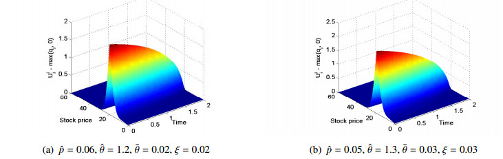
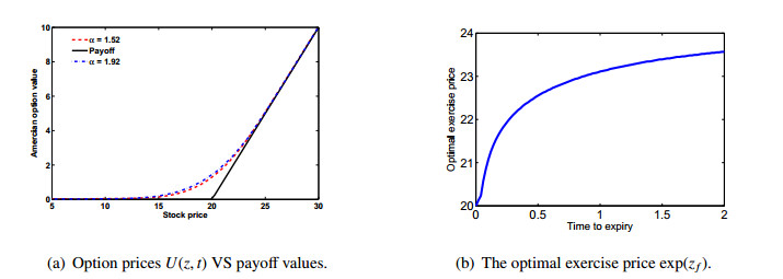
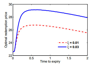
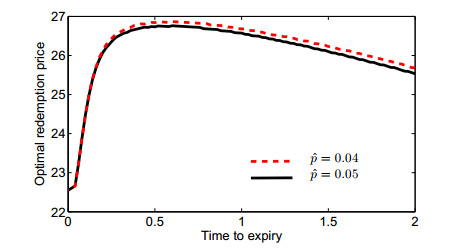
In this paper, the pricing of stock loans when the underlying follows a L$ \acute{e} $vy-$ \alpha $-stable process with jumps is considered. Under this complicated model, the stock loan value satisfies a fractional-partial-integro-differential equation (FPIDE) with a free boundary. The difficulties in solving the resulting FPIDE system are caused by the non-localness of the fractional-integro differential operator, together with the nonlinearity resulting from the early exercise opportunity of stock loans. Despite so many difficulties, we have managed to propose a preconditioned conjugate gradient normal residual (PCGNR) method to price efficiently the stock loan under such a complicated model. In the proposed approach, the moving pricing domain is successfully dealt with by introducing a penalty term, however, the semi-globalness of the fractional-integro operator is elegantly handled by the PCGNR method together with the fast Fourier transform (FFT) technique. Remarkably, we show both theoretically and numerically that the solution determined from the fixed domain problem by the current method is always above the intrinsic value of the corresponding option. Numerical experiments suggest the accuracy and advantage of the current approach over other methods that can be compared. Based on the numerical results, a quantitative discussion on the impacts of key parameters is also provided.
- Stock loans,
- L$ \acute{e} $vy-$ \alpha $-stable process,
- jump diffusions,
- fractional-partial-integro-differential equation,
- the PCGNR method
Citation: Congyin Fan, Wenting Chen, Bing Feng. Pricing stock loans under the L$ \acute{e} $vy-$ \alpha $-stable process with jumps[J]. Networks and Heterogeneous Media, 2023, 18(1): 191-211. doi: 10.3934/nhm.2023007

Related Papers:

Abstract

In this paper, the pricing of stock loans when the underlying follows a L$ \acute{e} $vy-$ \alpha $-stable process with jumps is considered. Under this complicated model, the stock loan value satisfies a fractional-partial-integro-differential equation (FPIDE) with a free boundary. The difficulties in solving the resulting FPIDE system are caused by the non-localness of the fractional-integro differential operator, together with the nonlinearity resulting from the early exercise opportunity of stock loans. Despite so many difficulties, we have managed to propose a preconditioned conjugate gradient normal residual (PCGNR) method to price efficiently the stock loan under such a complicated model. In the proposed approach, the moving pricing domain is successfully dealt with by introducing a penalty term, however, the semi-globalness of the fractional-integro operator is elegantly handled by the PCGNR method together with the fast Fourier transform (FFT) technique. Remarkably, we show both theoretically and numerically that the solution determined from the fixed domain problem by the current method is always above the intrinsic value of the corresponding option. Numerical experiments suggest the accuracy and advantage of the current approach over other methods that can be compared. Based on the numerical results, a quantitative discussion on the impacts of key parameters is also provided.

References

[1]	W. Chen, L. Xu, S. P. Zhu, Stock loan valuation under a stochstic interest rate model, Comput. Math. Appl., 70 (2015), 1757–1771. https://doi.org/10.1016/j.camwa.2015.07.019 doi: 10.1016/j.camwa.2015.07.019
[2]	J. Xia, X. Y. Zhou, Stock loans, Math. Financ., 17 (2007), 307–317. https://doi.org/10.1111/j.1467-9965.2006.00305.x doi: 10.1111/j.1467-9965.2006.00305.x
[3]	Z. Liang, W. Wu, S. Jiang, Stock loan with automatic termination clause, cap and margin, Comput. Math. Appl., 60 (2010), 3160–3176. https://doi.org/10.1016/j.camwa.2010.10.021 doi: 10.1016/j.camwa.2010.10.021
[4]	N. Cai, W. Zhang, Regime classification and stock loan valuation, Oper. Res., 68 (2020), 965–983. https://doi.org/10.1287/opre.2019.1934 doi: 10.1287/opre.2019.1934
[5]	M. Dai, Z. Q. Xu, Optimal redeeming strategy of stock loans with finite maturity, Math. Financ., 21 (2011), 775–793. https://doi.org/10.1111/j.1467-9965.2010.00449.x doi: 10.1111/j.1467-9965.2010.00449.x
[6]	X. Lu, E. R. M. Putri, Semi-analytic valuation of stock loans with finite maturity, Commun. Nonlinear. Sci., 27 (2015), 206–215. https://doi.org/10.1016/j.cnsns.2015.03.007 doi: 10.1016/j.cnsns.2015.03.007
[7]	D. Prager, Q. Zhang, Stock loan valuation under a regime-switching model with mean-reverting and finite maturity, J. Syst. Sci. Complex., 23 (2010), 572–583. https://doi.org/10.1007/s11424-010-0146-7 doi: 10.1007/s11424-010-0146-7
[8]	T. W. Wong, H. Y. Wong, Stochastic volatility asymptotics of stock loans: valuation and optimal stopping, J. Math. Anal. Appl., 394 (2012), 337–346. https://doi.org/10.1016/j.jmaa.2012.04.067 doi: 10.1016/j.jmaa.2012.04.067
[9]	Z. Zhou, J. Ma, X. Gao, Convergence of iterative Laplace transform methods for a system of fractional PDEs and PIDEs arising in option pricing, E. Asian. J. Appl. Math., 8 (2018), 782–808. https://doi.org/10.4208/eajam.130218.290618 doi: 10.4208/eajam.130218.290618
[10]	W. Chen, X. Xu, S. P. Zhu, Analytically pricing double barrier options based on a time-fractional Black-Scholes equation, Comput. Math. Appl., 69 (2015), 1407–1419. https://doi.org/10.1016/j.camwa.2015.03.025 doi: 10.1016/j.camwa.2015.03.025
[11]	P. Carr, H. Geman, D. B. Madan, Y. Marc, The fine structure of asset returns: an empirical investigation, J. Bus., 75 (2002), 305–332. https://doi.org/10.1086/338705 doi: 10.1086/338705
[12]	A. Cartea, D. del-Castillo-Negrete, Fractional diffusion models of option prices in markets with jumps, Physica A, 374 (2007), 749–763. https://doi.org/10.1016/j.physa.2006.08.071 doi: 10.1016/j.physa.2006.08.071
[13]	W. Chen, X. Xu, S. P. Zhu, Analytically pricing European-style options under the modified Black-Scholes equation with a spatial-fractional derivative, Q. Appl. Math., 72 (2014), 597–611. https://doi.org/10.1090/S0033-569X-2014-01373-2 doi: 10.1090/S0033-569X-2014-01373-2
[14]	W. Chen, M. Du, X. Xu, An explicit closed-form analytical solution for European options under the CGMY model, Commun. Nonlinear. Sci., 42 (2017), 285–297. https://doi.org/10.1016/j.cnsns.2016.05.026 doi: 10.1016/j.cnsns.2016.05.026
[15]	W. Chen, S. Lin, Option pricing under the KoBol model, Anziam. J., 60 (2018), 175–190. https://doi.org/10.1017/S1446181118000196 doi: 10.1017/S1446181118000196
[16]	W. Chen, X. Xu, S. P. Zhu, A predictor-corrector approach for pricing American options under the finite moment log-stable model, Appl. Numer. Math., 97 (2015), 15–29. https://doi.org/10.1016/j.apnum.2015.06.004 doi: 10.1016/j.apnum.2015.06.004
[17]	X. M. Gu, T. Z. Huang, C. C. Ji, B. Carpentieri, A. A. Alikhanov, Fast iterative method with a second-order implicit difference scheme for time-space fractional convection-diffusion equation. J. Sci. Comput., 72 (2017): 957–985. https://doi.org/10.1007/s10915-017-0388-9 doi: 10.1007/s10915-017-0388-9
[18]	X. M. Gu, Y. L. Zhao, X. L. Zhao, B. Carpentieri, Y. Y. Huang, A note on parallel preconditioning for the all-at-once solution of Riesz fractional diffusion equations, Numer. Math-Theory. Me., 14 (2021): 893–919. https://doi.org/10.48550/arXiv.2003.07020 doi: 10.48550/arXiv.2003.07020
[19]	X. Chen, D. Ding, S. L. Lei, W. Wang, A fast preconditioned iterative method for two-dimensional options pricing under fractional differential models. Comput. Math. Appl., 79 (2020): 440–456. https://doi.org/10.1016/j.camwa.2019.07.010 doi: 10.1016/j.camwa.2019.07.010
[20]	S. L. Lei, W. Wang, X. Chen, D. Ding, A fast preconditioned penalty method for American options pricing under regime-switching tempered fractional diffusion models, J. Sci. Comput., 75 (2018): 1633–1655. https://doi.org/10.1007/s10915-017-0602-9 doi: 10.1007/s10915-017-0602-9
[21]	W. Wang, X. Chen, D. Ding, S. L. Lei, Circulant preconditioning technique for barrier options pricing under fractional diffusion models, Int. J. Comput. Math., 92 (2015): 2596–2614. http://dx.doi.org/10.1080/00207160.2015.1077948 doi: 10.1080/00207160.2015.1077948
[22]	X. Chen, W. Wang, D. Ding, S. L. Lei, A fast preconditioned policy iteration method for solving the tempered fractional HJB equation governing American options valuation, Comput. Math. Appl., 73 (2017): 1932–1944. http://dx.doi.org/10.1016/j.camwa.2017.02.040 doi: 10.1016/j.camwa.2017.02.040
[23]	S. G. Kou, A jump-diffusion model for option pricing, Manage. Sci., 48 (2002), 1086–1101. https://doi.org/10.1287/mnsc.48.8.1086.166 doi: 10.1287/mnsc.48.8.1086.166
[24]	B. F. Nielsen, O. Skavhaug, A. Tveito, Penalty and front-fixing methods for the numerical solution of American option problems, J. Comput. Financ., 4 (2002), 69–97. https://doi.org/10.21314/jcf.2002.084 doi: 10.21314/jcf.2002.084
[25]	S. Chen, F. Liu, X. Jiang, I. Turner, V. Anh, A fast semi-implicit difference method for a nonlinear two-sided space-fractional diffusion equation with variable diffusivity coefficients, Appl. Math. Comput., 257 (2015), 591–601. https://doi.org/10.1016/j.amc.2014.08.031 doi: 10.1016/j.amc.2014.08.031
[26]	H. Hejazi, T. Moroney, F. Liu, Stability and convergence of a finite volume method for the space fractional advection-dispersion equation, J. Comput. Appl. Math., 255 (2014), 684–697. https://doi.org/10.1016/j.cam.2013.06.039 doi: 10.1016/j.cam.2013.06.039
[27]	O. Marom, E. Momoniat, A comparison of numerical solutions of fractional diffusion models in finance, Nonlinear. Anal-Real., 10 (2009), 3435–3442. https://doi.org/10.1016/j.nonrwa.2008.10.066 doi: 10.1016/j.nonrwa.2008.10.066
[28]	N. Cai, S. G. Kou, Option pricing under a mixed-exponential jump diffusion model, Manage. Sci., 57 (2011), 2067–2081. https://doi.org/10.1287/mnsc.1110.1393 doi: 10.1287/mnsc.1110.1393
[29]	Y. L. Zhao, P. Y. Zhu, X. M. Gu, X. L. Zhao, H. Y. Jian, A preconditioning technique for all-at-once system from the nonlinear tempered fractional diffusion equation, J. Sci. Comput., 83 (2020): 10. https://doi.org/10.1007/s10915-020-01193-1 doi: 10.1007/s10915-020-01193-1
[30]	S. L. Lei, H. W. Sun, A circulant preconditioner for fractional diffusion equations, J. Comput. Phys., 242 (2013), 715–725. https://doi.org/10.1016/j.jcp.2013.02.025 doi: 10.1016/j.jcp.2013.02.025

Reader Comments

Your name:*

Email:*
© 2023 the Author(s), licensee AIMS Press. This is an open access article distributed under the terms of the Creative Commons Attribution License (http://creativecommons.org/licenses/by/4.0)