In classical epidemic models, a neglected aspect is the heterogeneity of disease transmission and progression linked to the viral load of each infected individual. Here, we investigate the interplay between the evolution of individuals' viral load and the epidemic dynamics from a theoretical point of view. We propose a stochastic particle model describing the infection transmission and the individual physiological course of the disease. Agents have a double microscopic state: a discrete label, that denotes the epidemiological compartment to which they belong and switches in consequence of a Markovian process, and a microscopic trait, measuring their viral load, that changes in consequence of binary interactions or interactions with a background. Specifically, we consider Susceptible–Infected–Removed–like dynamics where infectious individuals may be isolated and the isolation rate may depend on the viral load–sensitivity and frequency of tests. We derive kinetic evolution equations for the distribution functions of the viral load of the individuals in each compartment, whence, via upscaling procedures, we obtain macroscopic equations for the densities and viral load momentum. We perform then a qualitative analysis of the ensuing macroscopic model. Finally, we present numerical tests in the case of both constant and viral load–dependent isolation control.
Citation: Rossella Della Marca, Nadia Loy, Andrea Tosin. An SIR–like kinetic model tracking individuals' viral load[J]. Networks and Heterogeneous Media, 2022, 17(3): 467-494. doi: 10.3934/nhm.2022017
In classical epidemic models, a neglected aspect is the heterogeneity of disease transmission and progression linked to the viral load of each infected individual. Here, we investigate the interplay between the evolution of individuals' viral load and the epidemic dynamics from a theoretical point of view. We propose a stochastic particle model describing the infection transmission and the individual physiological course of the disease. Agents have a double microscopic state: a discrete label, that denotes the epidemiological compartment to which they belong and switches in consequence of a Markovian process, and a microscopic trait, measuring their viral load, that changes in consequence of binary interactions or interactions with a background. Specifically, we consider Susceptible–Infected–Removed–like dynamics where infectious individuals may be isolated and the isolation rate may depend on the viral load–sensitivity and frequency of tests. We derive kinetic evolution equations for the distribution functions of the viral load of the individuals in each compartment, whence, via upscaling procedures, we obtain macroscopic equations for the densities and viral load momentum. We perform then a qualitative analysis of the ensuing macroscopic model. Finally, we present numerical tests in the case of both constant and viral load–dependent isolation control.

| [1] |
F. Brauer, P. van den Driessche and J. Wu, Mathematical Epidemiology, Springer, Berlin, 2008. |
| [2] |
Effects of information–induced behavioural changes during the COVID–19 lockdowns: The case of Italy. Royal Society Open Science (2020) 7: 201635. 
|
| [3] |
C. Castillo-Chavez, Z. Feng and W. Huang, On the computation of $\mathcal{R}_0$ and its role on global stability, in Mathematical Approaches for Emerging and Reemerging Infectious Diseases: An Introduction, Springer, New York, 125 (2002), 229–250. |
| [4] |
CDC, Centers for Disease Control and Prevention, 2014–2016 Ebola outbreak in West Africa, https://www.cdc.gov/vhf/ebola/history/2014-2016-outbreak/index.html, 2016, (Accessed on April 2021). |
| [5] |
CDC, Centers for Disease Control and Prevention, Rubella–Laboratory Testing, https://www.cdc.gov/rubella/lab/rna-detection.html, 2020, (Accessed on June 2021). |
| [6] |
M. Cevik, K. Kuppalli, J. Kindrachuk and M. Peiris, Virology, transmission, and pathogenesis of SARS–CoV–2, British Medical Journal, 371 (2020), m3862. |
| [7] |
On the evolution of virulence and the relationship between various measures of mortality. Proceedings of the Royal Society of London B (2002) 269: 1317-1323.
|
| [8] |
G. Dimarco, L. Pareschi, G. Toscani and M. Zanella, Wealth distribution under the spread of infectious diseases, Physical Review E, 102 (2020), 022303, 14pp. |
| [9] |
Kinetic models for epidemic dynamics with social heterogeneity. Journal of Mathematical Biology (2021) 83: 1-32.
|
| [10] |
Backwards bifurcations and catastrophe in simple models of fatal diseases. Journal of Mathematical Biology (1998) 36: 227-248.
|
| [11] |
ECDC, European Centre for Disease Prevention and Control, Latest evidence on COVID–19 – Infection, https://www.ecdc.europa.eu/en/covid-19/latest-evidence/infection, 2020, (Accessed on June 2021). |
| [12] |
European Commission - eurostat, Deaths and crude death rate, https://ec.europa.eu/eurostat/databrowser/view/tps00029/default/table?lang=en, 2021, (Accessed on April 2021). |
| [13] |
European Commission - eurostat, Live births and crude birth rate, https://ec.europa.eu/eurostat/databrowser/view/TPS00204/bookmark/table?lang=en&bookmarkId=5b6e67ac-186d-4081-aa98-1453b77ec260, 2021, (Accessed on April 2021). |
| [14] |
SARS–CoV–2 viral load is associated with increased disease severity and mortality. Nature Communications (2020) 11: 5493.
|
| [15] |
A. Goyal, D. B. Reeves, E. F. Cardozo-Ojeda, J. T. Schiffer and B. T. Mayer, Viral load and contact heterogeneity predict SARS–CoV–2 transmission and super–spreading events, eLife, 10 (2021), e63537. |
| [16] |
J. Guckenheimer and P. Holmes, Nonlinear Oscillations, Dynamical Systems, and Bifurcations of Vector Fields, Springer, Berlin, 1983. |
| [17] |
Temporal dynamics in viral shedding and transmissibility of COVID–19. Nature Medicine (2020) 26: 672-675.
|
| [18] | A contribution to the mathematical theory of epidemics. Proceedings of the Royal Society of London A (1927) 115: 700-721. |
| [19] | (1961) Stability by Liapunov's Direct Method with Applications. New York–London: Academic Press. |
| [20] |
D. B. Larremore, B. Wilder, E. Lester, S. Shehata, J. M. Burke, J. A. Hay, M. Tambe, M. J. Mina and R. Parker, Test sensitivity is secondary to frequency and turnaround time for COVID–19 screening, Science Advances, 7 (2021), eabd5393. |
| [21] |
Viral loads and duration of viral shedding in adult patients hospitalized with influenza. The Journal of Infectious Diseases (2009) 200: 492-500.
|
| [22] |
Stability of a non–local kinetic model for cell migration with density dependent orientation bias. Kinetic and Related Models (2020) 13: 1007-1027.
|
| [23] |
Markov jump processes and collision–like models in the kinetic description of multi–agent systems. Communications in Mathematical Sciences (2020) 18: 1539-1568.
|
| [24] |
Boltzmann–type equations for multi–agent systems with label switching. Kinetic and Related Models (2021) 14: 867-894.
|
| [25] |
A viral load–based model for epidemic spread on spatial networks. Mathematical Biosciences and Engineering (2021) 18: 5635-5663.
|
| [26] |
MATLAB, Matlab release 2020a. The MathWorks, Inc., Natick, MA, 2020. |
| [27] | (2013) Interacting Multiagent Systems: Kinetic Equations and Monte Carlo Methods. Oxford: Oxford University Press. |
| [28] |
Measles viral load may reflect SSPE disease progression. Virology Journal (2006) 3: 49.
|
| [29] |
Reproduction numbers and sub–threshold endemic equilibria for compartmental models of disease transmission. Mathematical Biosciences (2002) 180: 29-48.
|
| [30] |
Statistical physics of vaccination. Physics Reports (2016) 664: 1-113.
|
| [31] |
WHO, World Health Organization, Severe acute respiratory syndrome (SARS), https://www.who.int/csr/don/archive/disease/severe_acute_respiratory_syndrome/en/, 2004, (Accessed on April 2021). |
| [32] |
WHO, World Health Organization, Diagnostic testing for SARS–CoV–2. Interim guidance., file:///C:/Users/rosde/AppData/Local/Temp/WHO-2019-nCoV-laboratory-2020.6-eng-1.pdf, 2020, (Accessed on May 2021). |
| [33] |
WHO, World Health Organization, Coronavirus disease (COVID–19) pandemic, https://www.who.int/emergencies/diseases/novel-coronavirus-2019, 2021, (Accessed on April 2021). |


Figures(5) / Tables(2)
Rossella Della Marca, Nadia Loy, Andrea Tosin. An SIR–like kinetic model tracking individuals' viral load[J]. Networks and Heterogeneous Media, 2022, 17(3): 467-494. doi: 10.3934/nhm.2022017

Epidemic dynamics in absence of isolation control (
Contour plot of the basic reproduction number
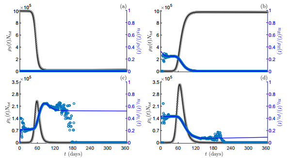
Viral load–dependent vs. constant isolation control. Numerical solutions as predicted by the model (16) (solid lines) and by the particle model (5) (markers) in scenarios S1 (grey scale colour) and S2 (blue scale colour). Panel (a): compartment size of infectious individuals with increasing viral load,
Viral load–dependent vs. constant isolation control. Numerical solutions as predicted by the model (16) (solid lines) and by the particle model (5) (markers) in scenarios S1 (grey scale colour) and S2 (blue scale colour). Panel (a): mean viral load of infectious individuals with increasing viral load,
Viral load evolution from the time of infection exposure to the final time


 DownLoad: