Mathematical analysis of transmission properties of electromagnetic meta-materials

Mario Ohlberger; Ben Schweizer; Maik Urban; Barbara Verfürth; Mario Ohlberger; Ben Schweizer; Maik Urban; Barbara Verfürth

doi:10.3934/nhm.2020002

Networks and Heterogeneous Media

2020, Volume 15, Issue 1: 29-56. doi: 10.3934/nhm.2020002

Previous Article Next Article

Mathematical analysis of transmission properties of electromagnetic meta-materials

1.
Angewandte Mathematik: Institut für Analysis und Numerik, Westfälische Wilhelms-Universität Münster, Einsteinstr. 62, DE-48149 Münster, Germany
2.
Fakultät für Mathematik, TU Dortmund, Vogelpothsweg 87, DE-44227 Dortmund, Germany
3.
Institut für Mathematik, Universität Augsburg, Universitätsstr. 14, DE-86159 Augsburg, Germany

Received: 01 September 2018 Revised: 01 October 2019
35B27, 35Q61, 65N30, 78M40

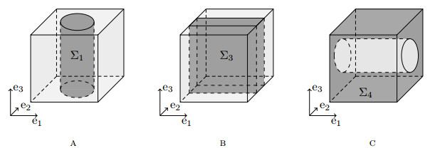
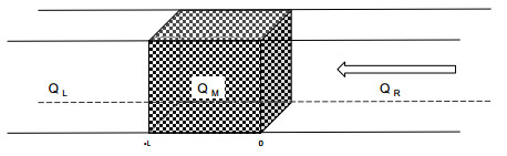
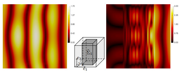
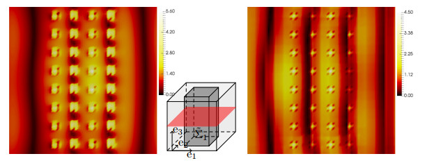
We study time-harmonic Maxwell's equations in meta-materials that use either perfect conductors or high-contrast materials. Based on known effective equations for perfectly conducting inclusions, we calculate the transmission and reflection coefficients for four different geometries. For high-contrast materials and essentially two-dimensional geometries, we analyze parallel electric and parallel magnetic fields and discuss their potential to exhibit transmission through a sample of meta-material. For a numerical study, one often needs a method that is adapted to heterogeneous media; we consider here a Heterogeneous Multiscale Method for high contrast materials. The qualitative transmission properties, as predicted by the analysis, are confirmed with numerical experiments. The numerical results also underline the applicability of the multiscale method.
- homogenization,
- Maxwell's equations,
- multiscale method,
- meta-material
Citation: Mario Ohlberger, Ben Schweizer, Maik Urban, Barbara Verfürth. Mathematical analysis of transmission properties of electromagnetic meta-materials[J]. Networks and Heterogeneous Media, 2020, 15(1): 29-56. doi: 10.3934/nhm.2020002

Related Papers:

Abstract

We study time-harmonic Maxwell's equations in meta-materials that use either perfect conductors or high-contrast materials. Based on known effective equations for perfectly conducting inclusions, we calculate the transmission and reflection coefficients for four different geometries. For high-contrast materials and essentially two-dimensional geometries, we analyze parallel electric and parallel magnetic fields and discuss their potential to exhibit transmission through a sample of meta-material. For a numerical study, one often needs a method that is adapted to heterogeneous media; we consider here a Heterogeneous Multiscale Method for high contrast materials. The qualitative transmission properties, as predicted by the analysis, are confirmed with numerical experiments. The numerical results also underline the applicability of the multiscale method.

References

[1]	On a priori error analysis of fully discrete heterogeneous multiscale FEM. Multiscale Model. Simul. (2005) 4: 447-459.
[2]	A generic grid interface for parallel and adaptive scientific computing. Ⅱ. Implementation and tests in DUNE. Computing (2008) 82: 121-138.
[3]	A generic grid interface for parallel and adaptive scientific computing. I. Abstract framework. Computing (2008) 82: 103-119.
[4]	Regularity of the Maxwell equations in heterogeneous media and Lipschitz domains. J. Math. Anal. Appl. (2013) 408: 498-512.
[5]	Multiscale nanorod metamaterials and realizable permittivity tensors. Commun. Comput. Phys. (2012) 11: 489-507.
[6]	Homogenization of the 3D Maxwell system near resonances and artificial magnetism. C. R. Math. Acad. Sci. Paris (2009) 347: 571-576.
[7]	Homogenization near resonances and artificial magnetism in three dimensional dielectric metamaterials. Arch. Ration. Mech. Anal. (2017) 225: 1233-1277.
[8]	Homogenization near resonances and artificial magnetism from dielectrics. C. R. Math. Acad. Sci. Paris (2004) 339: 377-382.
[9]	Homogenization of a wire photonic crystal: The case of small volume fraction. SIAM J. Appl. Math. (2006) 66: 2061-2084.
[10]	Homogenization of Maxwell's equations in a split ring geometry. Multiscale Model. Simul. (2010) 8: 717-750.
[11]	Plasmonic waves allow perfect transmission through sub-wavelength metallic gratings. Netw. Heterog. Media (2013) 8: 857-878.
[12]	Multiscale asymptotic method for Maxwell's equations in composite materials. SIAM J. Numer. Anal. (2010) 47: 4257-4289.
[13]	Homogenization of the system of high-contrast Maxwell equations. Mathematika (2015) 61: 475-500.
[14]	Asymptotic behaviour of the spectra of systems of Maxwell equations in periodic composite media with high contrast. Mathematika (2018) 64: 583-605.
[15]	High-dimensional finite elements for multiscale maxwell-type equations. IMA Journal of Numerical Analysis (2018) 38: 227-270.
[16]	Adaptive generalized multiscale finite element methods for H(curl)-elliptic problems with heterogeneous coefficients. J. Comput. Appl. Math. (2019) 345: 357-373.
[17]	On the approximation of electromagnetic fields by edge finite elements. Part 2: A heterogeneous multiscale method for Maxwell's equations. Comput. Math. Appl. (2017) 73: 1900-1919.
[18]	Singularities of electromagnetic fields in polyhedral domains. Arch. Ration. Mech. Anal. (2000) 151: 221-276.
[19]	Singularities of Maxwell interface problems. M2AN Math. Model. Numer. Anal. (1999) 33: 627-649.
[20]	Analysis of the heterogeneous multiscale method for elliptic homogenization problems. J. Amer. Math. Soc. (2005) 18: 121-156.
[21]	W. E and B. Engquist, The heterogeneous multiscale methods, Commun. Math. Sci., 1 (2003), 87–132, URL http://projecteuclid.org/euclid.cms/1118150402. doi: 10.4310/CMS.2003.v1.n1.a8
[22]	W. E and B. Engquist, The heterogeneous multi-scale method for homogenization problems, in Multiscale Methods in Science and Engineering, vol. 44 of Lect. Notes Comput. Sci. Eng., Springer, Berlin, 2005, 89–110. doi: 10.1007/3-540-26444-2_4
[23]	Dielectroc photonic crystal as medium with negative electric permittivity and magnetic permeability. Solid State Communications (2004) 129: 643-647.
[24]	Homogenization of a set of parallel fibres. Waves Random Media (1997) 7: 245-256.
[25]	Numerical homogenization of H(curl)-problems. SIAM J. Numer. Anal. (2018) 56: 1570-1596.
[26]	A new Heterogeneous Multiscale Method for time-harmonic Maxwell's equations. SIAM J. Numer. Anal. (2016) 54: 3493-3522.
[27]	M. Hochbruck and C. Stohrer, Finite element heterogeneous multiscale method for time-dependent Maxwell's equations, in Spectral and High Order Methods for Partial Differential Equations ICOSAHOM 2016 (eds. M. Bittencourt, N. Dumont and J. Hesthaven), vol. 119 of Lect. Notes Comput. Sci. Eng., Springer, Cham, 2017, 269–281, URL https://doi.org/10.1007/978-3-319-65870-4_18.
[28]	V. V. Jikov, S. M. Kozlov and O. A. Oleĭnik, Homogenization of Differential Operators and Integral Functionals, Springer-Verlag, Berlin, 1994, URL https://doi.org/10.1007/978-3-642-84659-5, Translated from the Russian by G. A. Yosifian. doi: 10.1007/978-3-642-84659-5
[29]	Two-scale homogenization for a general class of high contrast PDE systems with periodic coefficients. Applicable Analysis (2019) 98: 64-90.
[30]	A negative index meta-material for Maxwell's equations. SIAM J. Math. Anal. (2016) 48: 4155-4174.
[31]	Effective Maxwell equations in a geometry with flat rings of arbitrary shape. SIAM J. Math. Anal. (2013) 45: 1460-1494.
[32]	Effective Maxwell's equations for perfectly conducting split ring resonators. Arch. Ration. Mech. Anal. (2018) 229: 1197-1221.
[33]	C. Luo, S. G. Johnson, J. Joannopolous and J. Pendry, All-angle negative refraction without negative effective index, Phys. Rev. B, 65 (2002), 201104(R). doi: 10.1103/PhysRevB.65.201104
[34]	R. Milk and F. Schindler, dune-gdt, 2015, https://dx.doi.org/10.5281/zenodo.35389.
[35]	G. W. Milton, Realizability of metamaterials with prescribed electric permittivity and magnetic permeability tensors, New Journal of Physics, 12 (2010), 033035. doi: 10.1088/1367-2630/12/3/033035
[36]	(2003) Finite Element Methods for Maxwell's Equations. New York: Numerical Mathematics and Scientific Computation, Oxford University Press.
[37]	M. Ohlberger, A posteriori error estimates for the heterogeneous multiscale finite element method for elliptic homogenization problems, Multiscale Model. Simul., 4 (2005), 88–114 (electronic). doi: 10.1137/040605229
[38]	A new heterogeneous multiscale method for the Helmholtz equation with high contrast. Mulitscale Model. Simul. (2018) 16: 385-411.
[39]	A. Pokrovsky and A. Efros, Diffraction theory and focusing of light by a slab of left-handed material, Physica B: Condensed Matter, 338 (2003), 333–337, Proceedings of the Sixth International Conference on Electrical Transport and Optical Properties of Inhomogeneous Media. doi: 10.1016/j.physb.2003.08.015
[40]	Effective Maxwell's equations in general periodic microstructures. Applicable Analysis (2017) 97: 2210-2230.
[41]	Resonance meets homogenization: Construction of meta-materials with astonishing properties. Jahresber. Dtsch. Math.-Ver. (2017) 119: 31-51.
[42]	Propagation and localization of elastic waves in highly anisotropic periodic composites via two-scale homogenization. Mech. Mater. (2009) 41: 434-447.
[43]	Heterogeneous Multiscale method for the Maxwell equations with high contrast. ESAIM Math. Model. Numer. Anal. (2019) 53: 35-61.
[44]	On an extension and an application of the two-scale convergence method. Sbornik Mathematics (2000) 191: 973-1014.
[45]	On spectrum gaps of some divergent elliptic operators with periodic coefficients. St Petersburg Math. J. (2005) 16: 773-790.

Reader Comments

Your name:*

Email:*
© 2020 the Author(s), licensee AIMS Press. This is an open access article distributed under the terms of the Creative Commons Attribution License (http://creativecommons.org/licenses/by/4.0)