Gas flow through pipeline networks can be described using $ 2\times 2 $ hyperbolic balance laws along with coupling conditions at nodes. The numerical solution at steady state is highly sensitive to these coupling conditions and also to the balance between flux and source terms within the pipes. To avoid spurious oscillations for near equilibrium flows, it is essential to design well-balanced schemes. Recently Chertock, Herty & Özcan[
Citation: Yogiraj Mantri, Michael Herty, Sebastian Noelle. Well-balanced scheme for gas-flow in pipeline networks[J]. Networks and Heterogeneous Media, 2019, 14(4): 659-676. doi: 10.3934/nhm.2019026
Gas flow through pipeline networks can be described using $ 2\times 2 $ hyperbolic balance laws along with coupling conditions at nodes. The numerical solution at steady state is highly sensitive to these coupling conditions and also to the balance between flux and source terms within the pipes. To avoid spurious oscillations for near equilibrium flows, it is essential to design well-balanced schemes. Recently Chertock, Herty & Özcan[

| [1] |
A fast and stable well-balanced scheme with hydrostatic reconstruction for shallow water flows. SIAM J. Sci. Comput. (2004) 25: 2050-2065. 
|
| [2] |
Numerical discretization of coupling conditions by high-order schemes. J. Sci. Comput. (2016) 69: 122-145.
|
| [3] |
Coupling conditions for gas networks governed by the isothermal Euler equations. Netw. Heterog. Media (2006) 1: 295-314.
|
| [4] |
Gas flow in pipeline networks. Netw. Heterog. Media (2006) 1: 41-56.
|
| [5] |
Treating network junctions in finite volume solution of transient gas flow models. J. Comput. Phys. (2017) 344: 187-209.
|
| [6] |
A well-balanced reconstruction of wet/dry fronts for the shallow water equations. J. Sci. Comput. (2013) 56: 267-290.
|
| [7] |
ADER schemes and high order coupling on networks of hyperbolic conservation laws. J. Comput. Phys. (2014) 273: 658-670.
|
| [8] |
Flows on networks: Recent results and perspectives. EMS Surv. Math. Sci. (2014) 1: 47-111.
|
| [9] |
Gas pipeline models revisited: Model hierarchies, nonisothermal models, and simulations of networks. Multiscale Model. Simul. (2011) 9: 601-623.
|
| [10] |
A new hydrostatic reconstruction scheme based on subcell reconstructions. SIAM J. Numer. Anal. (2017) 55: 758-784.
|
| [11] | Well-balanced central-upwind schemes for $2\times 2$ system of balance laws. Theory, Numerics and Applications of Hyperbolic Problems. Ⅰ, Springer Proc. Math. Stat. Springer, Cham (2018) 236: 345-361. |
| [12] |
Optimal control in networks of pipes and canals. SIAM J. Control Optim. (2009) 48: 2032-2050.
|
| [13] |
On $2\times 2$ conservation laws at a junction. SIAM J. Math. Anal. (2008) 40: 605-622.
|
| [14] |
A well posed Riemann problem for the $p$-system at a junction. Netw. Heterog. Media (2006) 1: 495-511.
|
| [15] |
On the Cauchy problem for the $p$-system at a junction. SIAM J. Math. Anal. (2008) 39: 1456-1471.
|
| [16] |
Euler system for compressible fluids at a junction. J. Hyperbolic Differ. Equ. (2008) 5: 547-568.
|
| [17] |
R. Courant and K. O. Friedrichs, Supersonic Flow and Shock Waves, Interscience Publishers, Inc., New York, N. Y., 1948. |
| [18] |
Operator splitting method for simulation of dynamic flows in natural gas pipeline networks. Phys. D (2017) 361: 1-11.
|
| [19] |
H. Egger, A robust conservative mixed finite element method for isentropic compressible flow on pipe networks, SIAM J. Sci. Comput., 40 (2018), A108–A129. |
| [20] |
The numerical interface coupling of nonlinear hyperbolic systems of conservation laws. Ⅱ. The case of systems. M2AN Math. Model. Numer. Anal. (2005) 39: 649-692.
|
| [21] |
Coupling conditions for the transition from supersonic to subsonic fluid states. Netw. Heterog. Media (2017) 12: 371-380.
|
| [22] |
The isothermal Euler equations for ideal gas with source term: Product solutions, flow reversal and no blow up. J. Math. Anal. Appl. (2017) 454: 439-452.
|
| [23] |
A new model for gas flow in pipe networks. Math. Methods Appl. Sci. (2010) 33: 845-855.
|
| [24] |
Simulation of transient gas flow at pipe-to-pipe intersections. Internat. J. Numer. Methods Fluids (2008) 56: 485-506.
|
| [25] |
Semidiscrete central-upwind schemes for hyperbolic conservation laws and Hamilton-Jacobi equations. SIAM J. Sci. Comput. (2001) 23: 707-740.
|
| [26] |
New high-resolution central schemes for nonlinear conservation laws and convection-diffusion equations. J. Comput. Phys. (2000) 160: 241-282.
|
| [27] |
Pipe networks: Coupling constants in a junction for the isentropic euler equations. Energy Procedia (2015) 64: 140-149.
|
| [28] |
On a third order CWENO boundary treatment with application to networks of hyperbolic conservation laws. Appl. Math. Comput. (2018) 325: 252-270.
|
| [29] |
Well-balanced finite volume schemes of arbitrary order of accuracy for shallow water flows. J. Comput. Phys. (2006) 213: 474-499.
|
| [30] |
High-order well-balanced finite volume WENO schemes for shallow water equation with moving water. J. Comput. Phys. (2007) 226: 29-58.
|
| [31] |
Nonlinear programming applied to the optimum control of a gas compressor station. Internat. J. Numer. Methods Engrg. (1980) 15: 1287-1301.
|
| [32] |
G. Puppo and G. Russo, Numerical Methods for Balance Laws, Quaderni di Matematica, 24. Department of Mathematics, Seconda Università di Napoli, Caserta, 2009. |
| [33] |
Numerical network models and entropy principles for isothermal junction flow. Netw. Heterog. Media (2014) 9: 65-95.
|
| [34] |
Existence and uniqueness of solutions to the generalized {R}iemann problem for isentropic flow. SIAM J. Appl. Math. (2015) 75: 679-702.
|
| [35] |
Coupling constants and the generalized Riemann problem for isothermal junction flow. J. Hyperbolic Differ. Equ. (2015) 12: 37-59.
|


Figures(8) / Tables(2)
Yogiraj Mantri, Michael Herty, Sebastian Noelle. Well-balanced scheme for gas-flow in pipeline networks[J]. Networks and Heterogeneous Media, 2019, 14(4): 659-676. doi: 10.3934/nhm.2019026

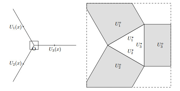
Intersection of three pipes at junction O. Right-Zoomed view of the junction with old traces
Phase plot in terms of equilibrium variables with initial state
Momentum for perturbation of order
Momentum for perturbation of order
Momentum for perturbation of order
Momentum for perturbation of order
Conservative variables,
Conservative variables,


 DownLoad: