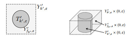
We consider the Stokes system in a thin porous medium $ \Omega_\varepsilon $ of thickness $ \varepsilon $ which is perforated by periodically distributed solid cylinders of size $ \varepsilon $. On the boundary of the cylinders we prescribe non-homogeneous slip boundary conditions depending on a parameter $ \gamma $. The aim is to give the asymptotic behavior of the velocity and the pressure of the fluid as $ \varepsilon $ goes to zero. Using an adaptation of the unfolding method, we give, following the values of $ \gamma $, different limit systems.
Citation: María Anguiano, Francisco Javier Suárez-Grau. Newtonian fluid flow in a thin porous medium with non-homogeneous slip boundary conditions[J]. Networks and Heterogeneous Media, 2019, 14(2): 289-316. doi: 10.3934/nhm.2019012
We consider the Stokes system in a thin porous medium $ \Omega_\varepsilon $ of thickness $ \varepsilon $ which is perforated by periodically distributed solid cylinders of size $ \varepsilon $. On the boundary of the cylinders we prescribe non-homogeneous slip boundary conditions depending on a parameter $ \gamma $. The aim is to give the asymptotic behavior of the velocity and the pressure of the fluid as $ \varepsilon $ goes to zero. Using an adaptation of the unfolding method, we give, following the values of $ \gamma $, different limit systems.

| [1] |
Self-assembly of block copolymer thin films. Materials Today (2010) 13: 24-33. 
|
| [2] |
Homogenization of the Navier-Stokes equations with a slip boundary condition. Comm. Pure Appl. Math. (1989) 44: 605-642.
|
| [3] |
Homogenization and two-scale convergence. SIAM J. Math. Anal. (1992) 23: 1482-1518.
|
| [4] |
M. Anguiano and F. J. Suárez-Grau, Homogenization of an incompressible non-Newtonian flow through a thin porous medium, Z. Angew. Math. Phys., 68 (2017), Art. 45, 25 pp. doi: 10.1007/s00033-017-0790-z
|
| [5] |
Derivation of the double porosity model of single phase flow via homogenization theory. SIAM J. Math. Anal. (1990) 21: 823-836.
|
| [6] |
Convergence of the homogenization process for a double-porosity model of immiscible two-phase flow. SIAM J. Math.Anal. (1996) 27: 1520-1543.
|
| [7] |
Homogenisation of the Stokes problem with a pure non-homogeneous slip boundary condition by the periodic unfolding method. Euro. J. of Applied Mathematics (2011) 22: 333-345.
|
| [8] |
Homogenization in open sets with holes. J. Math. Anal. Appl. (1979) 71: 590-607.
|
| [9] | Homogénéisation du problème du Neumann non homogène dans des ouverts perforés. Asymptotic Analysis (1988) 1: 115-138. |
| [10] | Exact internal controllability in perforated domains. J. Math. Pures Appl. (1989) 68: 185-213. |
| [11] |
D. Cioranescu and J. Saint Jean Paulin, Truss structures: Fourier conditions and eigenvalue problems, in Boundary Control and Boundary Variation (Ed. J.P. Zolezio), Springer-Verlag, 178 (1992), 125-141. doi: 10.1007/BFb0006691
|
| [12] |
Homogenization of the Stokes problem with non homogeneous slip boundary conditions. Math. Meth. Appl. Sci. (1996) 19: 857-881.
|
| [13] |
Periodic unfolding and homogenization. C.R. Acad. Sci. Paris Ser. I (2002) 335: 99-104.
|
| [14] |
Periodic unfolding and Robin problems in perforated domains. C. R. Math. (2006) 342: 469-474.
|
| [15] | The periodic unfolding method in perforated domains. Portugaliae Mathematica (2006) 63: 467-496. |
| [16] |
The periodic unfolding method in domains with holes. SIAM J. of Math. Anal. (2012) 44: 718-760.
|
| [17] | On the application of the homogenization theory to a class of problems arising in fluid mechanics. J. Math. Pures Appl. (1985) 64: 31-75. |
| [18] | The period unfolding method for the wave equations in domains with holes. Advances in Mathematical Sciences and Applications (2012) 22: 521-551. |
| [19] |
The periodic unfolding method for the heat equation in perforated domains. Science China Mathematics (2016) 59: 891-906.
|
| [20] | Equation et phénomenes de surface pour l'écoulement dans un modèle de milieux poreux. J. Mech. (1975) 14: 73-108. |
| [21] |
Chemical Interactions and Their Role in the Microphase Separation of Block Copolymer Thin Films. Int. J. of Molecular Sci. (2009) 10: 3671-3712.
|
| [22] |
Lattice gas analysis of liquid front in non-crimp fabrics. Transp. Porous Med. (2011) 84: 75-93.
|
| [23] |
Design and simulation of passive mixing in microfluidic systems with geometric variations. Chem. Eng. J. (2009) 152: 575-582.
|
| [24] | J.-L. Lions and E. Magenes, Problèmes aux Limites non Homogènes et Applications, Dunod, Paris, 1968. |
| [25] | Measurements of the permeability tensor of compressed fibre beds. Transp. Porous Med. (2002) 47: 363-380. |
| [26] | Two-scale convergence for thin domain and its applications to some lower-dimensional model in fluid mechanics. Asymptot. Anal. (2000) 23: 23-57. |
| [27] | J. Nečas, Les méthodes Directes en Théorie des Équations Elliptiques, Masson, Paris, 1967. |
| [28] |
A general convergence result for a functional related to the theory of homogenization. SIAM J. Math. Anal. (1989) 20: 608-623.
|
| [29] |
Effect of multi-scale porosity in local permeability modelling of non-crimp fabrics. Transp. Porous Med. (2008) 73: 109-124.
|
| [30] |
Enabling nanotechnology with self assembled block copolymer patterns. Polymer (2003) 44: 6725-6760.
|
| [31] | F. F. Reuss, Notice sur un Nouvel Effet de L'electricité Galvanique, Mémoire Soc. Sup. Imp. de Moscou, 1809. |
| [32] | E. Sanchez-Palencia, Non-Homogeneous Media and Vibration Theory, Lecture Notes in Physics, 127. Springer-Verlag, Berlin-New York, 1980. |
| [33] |
Micro-PIV measurement of flow upstream of papermaking forming fabrics. Transp. Porous Med. (2015) 107: 435-448.
|
| [34] | Multiscale modeling of unsaturated flow in dual-scale fiber preforms of liquid composite molding I: Isothermal flows. Compos. Part A Appl. Sci. Manuf. (2012) 43: 1-13. |
| [35] | L. Tartar, Incompressible fluid flow in a porous medium convergence of the homogenization process., in Appendix to Lecture Notes in Physics, 127 (1980). |
| [36] |
Homogenization of eigenvalues problems in perforated domains. Proc. Indian Acad. of Science (1981) 90: 239-271.
|
| [37] | Homogenization of a Stokes problem in a porous medium by the periodic unfolding method. Asymptotic Analysis (2012) 79: 229-250. |


Figures(3)
María Anguiano, Francisco Javier Suárez-Grau. Newtonian fluid flow in a thin porous medium with non-homogeneous slip boundary conditions[J]. Networks and Heterogeneous Media, 2019, 14(2): 289-316. doi: 10.3934/nhm.2019012


 DownLoad: