This work deals with a mathematical analysis of sodium's transport in a tubular architecture of a kidney nephron. The nephron is modelled by two counter-current tubules. Ionic exchange occurs at the interface between the tubules and the epithelium and between the epithelium and the surrounding environment (interstitium). From a mathematical point of view, this model consists of a 5$ \times $5 semi-linear hyperbolic system. In literature similar models neglect the epithelial layers. In this paper, we show rigorously that such models may be obtained by assuming that the permeabilities between lumen and epithelium are large. We show that when these permeabilities grow, solutions of the 5$ \times $5 system converge to those of a reduced 3$ \times $3 system without epithelial layers. The problem is defined on a bounded spacial domain with initial and boundary data. In order to show convergence, we use $ {{{\rm{BV}}}} $ compactness, which leads to introduce initial layers and to handle carefully the presence of lateral boundaries. We then discretize both 5$ \times $5 and 3$ \times $3 systems, and show numerically the same asymptotic result, for a fixed meshsize.
Citation: Marta Marulli, Vuk Miliši$\grave{\rm{c}}$, Nicolas Vauchelet. Reduction of a model for sodium exchanges in kidney nephron[J]. Networks and Heterogeneous Media, 2021, 16(4): 609-636. doi: 10.3934/nhm.2021020
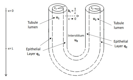
This work deals with a mathematical analysis of sodium's transport in a tubular architecture of a kidney nephron. The nephron is modelled by two counter-current tubules. Ionic exchange occurs at the interface between the tubules and the epithelium and between the epithelium and the surrounding environment (interstitium). From a mathematical point of view, this model consists of a 5$ \times $5 semi-linear hyperbolic system. In literature similar models neglect the epithelial layers. In this paper, we show rigorously that such models may be obtained by assuming that the permeabilities between lumen and epithelium are large. We show that when these permeabilities grow, solutions of the 5$ \times $5 system converge to those of a reduced 3$ \times $3 system without epithelial layers. The problem is defined on a bounded spacial domain with initial and boundary data. In order to show convergence, we use $ {{{\rm{BV}}}} $ compactness, which leads to introduce initial layers and to handle carefully the presence of lateral boundaries. We then discretize both 5$ \times $5 and 3$ \times $3 systems, and show numerically the same asymptotic result, for a fixed meshsize.

| [1] |
Human nephron number: Implications for health and disease. Pediatr. Nephrol. (2011) 26: 1529-1533. 
|
| [2] |
J. S. Clemmer, W. A. Pruett, T. G. Coleman, J. E. Hall and R. L. Hester, Mechanisms of blood pressure salt sensitivity: New insights from mathematical modeling, Am. J. Physiol. Regul. Integr. Comp. Physiol., 312 (2016), R451–R466. doi: 10.1152/ajpregu.00353.2016
|
| [3] |
C. M. Dafermos, Hyperbolic Conservation Laws in Continuum Physics, 4th edition, volume 325, Berlin: Springer, 2016. doi: 10.1007/978-3-662-49451-6
|
| [4] | A. Edwards, M. Auberson, S. Ramakrishnan and O. Bonny, A model of uric acid transport in the rat proximal tubule, Am. J. Physiol. Renal Physiol., (2019), F934–F947. |
| [5] |
Impact of nitric-oxide-mediated vasodilation and oxidative stress on renal medullary oxygenation: A modeling study. Am. J. Physiol. Renal Physiol. (2016) 310: F237-F247.
|
| [6] |
V. Giovangigli, Z.-B. Yang and W.-A. Yong, Relaxation limit and initial-layers for a class of hyperbolic-parabolic systems, SIAM J. Math. Anal., 50 (2018), 4655–4697. doi: 10.1137/18M1170091
|
| [7] |
E. Giusti, Minimal Surfaces and Functions of Bounded Variation, volume 80., Birkhäuser/Springer, Basel, 1984. doi: 10.1007/978-1-4684-9486-0
|
| [8] | E. Godlewski and P.-A. Raviart, Hyperbolic Systems of Conservation Laws, volume 3/4., Paris: Ellipses, 1991. |
| [9] |
A quantitative systems physiology model of renal function and blood pressure regulation: Application in salt-sensitive hypertension. CPT Pharmacometrics Syst. Pharmacol. (2017) 6: 393-400.
|
| [10] |
The multiplication principle as the basis for concentrating urine in the kidney. Journal of the American Society of Nephrology (2001) 12: 1566-1586.
|
| [11] |
M. Heida, R. I. A. Patterson and D. R. M. Renger, Topologies and measures on the space of functions of bounded variation taking values in a Banach or metric space, J. Evol. Equ., 19 (2019), 111–152. doi: 10.1007/s00028-018-0471-1
|
| [12] |
F. James, Convergence results for some conservation laws with a reflux boundary condition and a relaxation term arising in chemical engineering, SIAM J. Math. Anal., 29 (1998), 1200–1223. doi: 10.1137/S003614109630793X
|
| [13] |
S. Jin and Z. Xin, The relaxation schemes for systems of conservation laws in arbitrary space dimensions, Commun. Pure Appl. Math., 48 (1995), 235–276. doi: 10.1002/cpa.3160480303
|
| [14] |
A computational model for simulating solute transport and oxygen consumption along the nephrons. Am. J. Physiol. Renal Physiol. (2016) 311: F1378-F1390.
|
| [15] |
Mathematical modeling of kidney transport. Wiley Interdiscip Rev. Syst. Biol. Med. (2013) 5: 557-573.
|
| [16] |
A. T. Layton and A. Edwards, Mathematical Modeling in Renal Physiology, Springer, 2014. doi: 10.1007/978-3-642-27367-4
|
| [17] |
Distribution of henle's loops may enhance urine concentrating capability. Biophys. J. (1986) 49: 1033-1040.
|
| [18] |
P. G. LeFloch, Hyperbolic Systems of Conservation Laws. The Theory of Classical and Nonclassical Shock Waves, Basel: Birkhäuser, 2002. doi: 10.1007/978-3-0348-8150-0
|
| [19] |
M. Marulli, A. Edwards, V. Milišić and N. Vauchelet, On the role of the epithelium in a model of sodium exchange in renal tubules, Math. Biosci., 321 (2020), 108308, 12 pp. doi: 10.1016/j.mbs.2020.108308
|
| [20] |
V. Milišić and D. Oelz, On the asymptotic regime of a model for friction mediated by transient elastic linkages, J. Math. Pures Appl. (9), 96 (2011), 484–501. doi: 10.1016/j.matpur.2011.03.005
|
| [21] |
Hormonal regulation of salt and water excretion: A mathematical model of whole kidney function and pressure natriuresis. Am. J. Physiol. Renal Physiol. (2014) 306: F224-F248.
|
| [22] |
R. Natalini and A. Terracina, Convergence of a relaxation approximation to a boundary value problem for conservation laws, Comm. Partial Differential Equations, 26 (2001), 1235–1252. doi: 10.1081/PDE-100106133
|
| [23] | Transport efficiency and workload distribution in a mathematical model of the thick ascending limb. Am. J. Physiol. Renal Physiol. (2012) 304: F653-F664. |
| [24] | B. Perthame, Transport Equations Biology, Basel: Birkhäuser, 2007. |
| [25] |
B. Perthame, N. Seguin and M. Tournus, A simple derivation of BV bounds for inhomogeneous relaxation systems, Commun. Math. Sci., 13 (2015), 577–586. doi: 10.4310/CMS.2015.v13.n2.a17
|
| [26] | J. L. Stephenson, Urinary Concentration and Dilution: Models, American Cancer Society, (2011), 1349–1408. |
| [27] | M. Tournus, Modèles D'échanges Ioniques Dans le Rein: Théorie, Analyse Asymptotique et Applications Numériques, PhD thesis, Université Pierre et Marie Curie, France, 2013. |
| [28] |
M. Tournus, A. Edwards, N. Seguin and B. Perthame, Analysis of a simplified model of the urine concentration mechanism, Netw. Heterog. Media, 7 (2012), 989–1018. doi: 10.3934/nhm.2012.7.989
|
| [29] |
A model of calcium transport along the rat nephron. Am. J. Physiol. Renal Physiol. (2013) 305: F979-F994.
|
| [30] |
A mathematical model of the rat nephron: Glucose transport. Am. J. Physiol. Renal Physiol. (2015) 308: F1098-F1118.
|
| [31] |
A mathematical model of the rat kidney: K$^{+}$-induced natriuresis. Am. J. Physiol. Renal Physiol. (2017) 312: F925-F950.
|
| [32] |
W. P. Ziemer, Weakly Differentiable Functions. Sobolev Spaces and Functions of Bounded Variation, Graduate Texts in Mathematics, 120. Springer-Verlag, New York, 1989. doi: 10.1007/978-1-4612-1015-3
|

Figures(2)
Marta Marulli, Vuk Miliši$\grave{\rm{c}}$, Nicolas Vauchelet. Reduction of a model for sodium exchanges in kidney nephron[J]. Networks and Heterogeneous Media, 2021, 16(4): 609-636. doi: 10.3934/nhm.2021020


 DownLoad: