Existence and stability of solutions for Hadamard type fractional differential systems with $ p $-Laplacian operators on benzoic acid graphs

Yunzhe Zhang; Youhui Su; Yongzhen Yun; Yunzhe Zhang; Youhui Su; Yongzhen Yun

doi:10.3934/math.2025356

AIMS Mathematics

2025, Volume 10, Issue 4: 7767-7794. doi: 10.3934/math.2025356

Previous Article Next Article

Research article Special Issues

Existence and stability of solutions for Hadamard type fractional differential systems with $ p $-Laplacian operators on benzoic acid graphs

1.
School of Mathematics and Statistics, Xuzhou University of Technology, Xuzhou 221018, Jiangsu, China
2.
School of Science, Shenyang University of Technology, Shenyang 110870, Liaoning, China

Received: 13 February 2025 Revised: 19 March 2025 Accepted: 24 March 2025 Published: 02 April 2025
MSC : 34A08, 34B15, 34K37

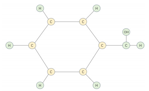
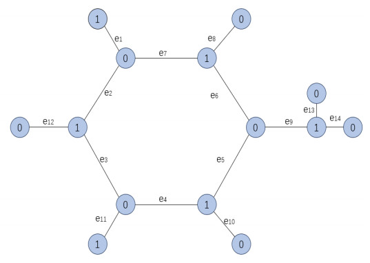
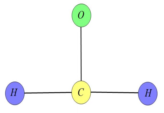
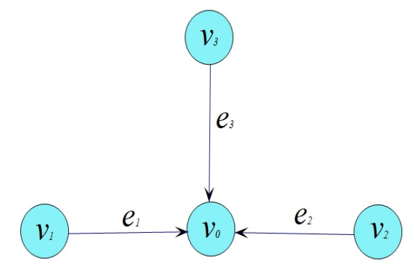
Benzoic acid is mainly used in the preparation of sodium benzoate preservatives, as well as in the synthesis of drugs and dyes. Therefore, a thorough understanding of its properties is of utmost importance. This paper is mainly concerned with the existence of solutions for a class of Hadamard type fractional differential systems with $ p $-Laplacian operators on benzoic acid graphs. Meanwhile, the Hyers-Ulam stability of the systems is also proved. Furthermore, an example is presented on a formaldehyde graph to demonstrate the applicability of the conclusions obtained. The novelty of this paper lies in the integration of fractional differential equations with graph theory, utilizing the formaldehyde graph as a specific case for numerical simulation, and providing an approximate solution graph after iterations.
- fractional differential equation,
- benzoic acid graphs,
- Hyers-Ulam stability,
- numerical simulation
Citation: Yunzhe Zhang, Youhui Su, Yongzhen Yun. Existence and stability of solutions for Hadamard type fractional differential systems with $ p $-Laplacian operators on benzoic acid graphs[J]. AIMS Mathematics, 2025, 10(4): 7767-7794. doi: 10.3934/math.2025356

Related Papers:

Abstract

Benzoic acid is mainly used in the preparation of sodium benzoate preservatives, as well as in the synthesis of drugs and dyes. Therefore, a thorough understanding of its properties is of utmost importance. This paper is mainly concerned with the existence of solutions for a class of Hadamard type fractional differential systems with $ p $-Laplacian operators on benzoic acid graphs. Meanwhile, the Hyers-Ulam stability of the systems is also proved. Furthermore, an example is presented on a formaldehyde graph to demonstrate the applicability of the conclusions obtained. The novelty of this paper lies in the integration of fractional differential equations with graph theory, utilizing the formaldehyde graph as a specific case for numerical simulation, and providing an approximate solution graph after iterations.

References

[1]	A. Sun, Y. Su, Q. Yuan, T. Li, Existence of solutions to fractional differential equations with fractional order derivative terms, J. Appl. Anal. Comput., 11 (2021), 486–520. http://dx.doi.org/10.11948/20200072 doi: 10.11948/20200072
[2]	R. Hilfer, Applications of fractional calculus in physics, 1 Eds., Singapore: World Scientific, 2000. http://dx.doi.org/10.1142/3779
[3]	V. Lakshmikanthan, A. S. Vatsala, Basic theory of fractional differential equations, Nonlinear Anal., 69 (2008), 267–782. http://dx.doi.org/10.1016/j.na.2007.08.042 doi: 10.1016/j.na.2007.08.042
[4]	M. A. Krasnoselskii, Two remarks on the method of successive approximations, Russian Math. Surveys, 10 (1955), 123–127.
[5]	W. Sun, Y. Su, X. Han, Existence of solutions for a coupled system of Caputo-Hadamard fractional differential equations with $p$-Laplacian operator, J. Appl. Anal. Comput., 12 (2022), 1885–1900. http://dx.doi.org/10.11948/20210384 doi: 10.11948/20210384
[6]	Y. Cu, W. Ma, Q. Sun, X. Su, New uniqueness results for boundary value problem of fractional differential equation, Nonlinear Anal. Model. Control, 23 (2018), 31–39. http://dx.doi.org/10.15388/na.2018.1.3 doi: 10.15388/na.2018.1.3
[7]	M. Faieghi, S. Kuntanapreeda, H. Delavari, D. Baleanu, LMI-based stabilization of a class of fractional-order chaotic systems, Nonlinear Dyn., 72 (2013), 301–309. http://dx.doi.org/10.1007/s11071-012-0714-6 doi: 10.1007/s11071-012-0714-6
[8]	D. Tripathil, S. K. Pandey, S. Das, Peristaltic flow of viscoelastic fluid with fractional maxwell model through a channel, Appl. Math. Comput., 215 (2010), 3645–3654. http://dx.doi.org/10.1016/j.amc.2009.11.002 doi: 10.1016/j.amc.2009.11.002
[9]	Y. Jalilian, Fractional integral inequalities and their applications to fractional differential equations, Acta Math. Sci., 36 (2016), 1317–1330. http://dx.doi.org/10.1016/S0252-9602(16)30071-6 doi: 10.1016/S0252-9602(16)30071-6
[10]	A. Turab, W. Sintunavarat, The novel existence results of solutions for a nonlinear fractional boundary value problem on the ethane graph, Alexandria Eng. J., 60 (2021), 5365–5374. http://dx.doi.org/10.1016/j.aej.2021.04.020 doi: 10.1016/j.aej.2021.04.020
[11]	A. Z. Abdian, A. Behmaram, G. H. Fath-Tabar, Graphs determined by signless Laplacian spectra, Akce. Int. J. Graphs Co., 17 (2020), 45–50. https://doi.org/10.1016/j.akcej.2018.06.009 doi: 10.1016/j.akcej.2018.06.009
[12]	R. Ch. Kulaev, A. A. Urtaeva, On the existence of a boundary value problem on a graph for a nonlinear equation of the forth order, Diff. Equat., 59 (2023), 1175–1184. http://dx.doi.org/10.1134/S0012266123090033 doi: 10.1134/S0012266123090033
[13]	A. M. S. Mahdy, M. S. Mohamed, K. A. Gepreel, A. AL-Amiri, M. Higazy, Dynamical characteristics and signal flow graph of nonlinear fractional smoking mathematical model, Chaos Soliton Fract., 141 (2020), 110308. http://dx.doi.org/10.1016/j.chaos.2020.110308 doi: 10.1016/j.chaos.2020.110308
[14]	J. R. Graef, L. Kong, M. Wang, Existence and uniqueness of solutions for a fractional boundary value problem on a graph, Fract. Calc. Appl. Anal., 17 (2014), 499–510. http://dx.doi.org/10.2478/s13540-014-0182-4 doi: 10.2478/s13540-014-0182-4
[15]	V. Mehandiratta, M. Mehra, G. Leugering, Existence and uniqueness results for a nonlinear Caputo fractional boundary value problem on a star graph, J. Math. Anal. Appl., 477 (2019), 1243–1264. http://dx.doi.org/10.1016/j.jmaa.2019.05.011 doi: 10.1016/j.jmaa.2019.05.011
[16]	W. Zhang, W. Liu, Existence and Ulam's type stability results for a class of fractional boundary value problems on a star graph, Math. Method. Appl. Sci., 43 (2020), 8568–8594. http://dx.doi.org/10.1002/mma.6516 doi: 10.1002/mma.6516
[17]	J. R. Wang, Y. Zhou, M. Medve, Existence and stability of fractional differential equations with Hadamard derivative, Topol. Methods Nonlinear Anal., 41 (2013), 113–133.
[18]	B. Ahmad, M. Alghanmi, A. Alsaedi, J. J. Nieto, Existence and uniqueness results for a nonlinear coupled system involving Caputo fractional derivatives with a new kind of coupled boundary conditions, Appl. Math. Lett., 116 (2021), 107018. http://dx.doi.org/10.1016/j.aml.2021.107018 doi: 10.1016/j.aml.2021.107018
[19]	N. A. Sheikh, M. Jamil, D. L. C. Ching, I. Khan, M. Usman, K. S. Nisar, A generalized model for quantitative analysis of sediments loss: A Caputo time fractional model, J. King. Saud Univ. Sci., 33 (2020), 101179. http://dx.doi.org/10.1016/j.jksus.2020.09.006 doi: 10.1016/j.jksus.2020.09.006
[20]	B. Ahmad, A. Alsaedi, S. K. Ntouyas, J. Tariboon, Hadamard-type fractional differential equations, inclusions and inequalities, 1 Eds., Cham: Springer, 2017. http://dx.doi.org/10.1007/978-3-319-52141-1
[21]	H. Aktuǧlu, M. A. Özarslan, Solvability of differential equations of order $2 < \alpha\leq3$ involving the $p$-Laplacian operator with boundary conditions, Adv. Differ. Equ., 2013 (2013), 358. http://dx.doi.org/10.1186/1687-1847-2013-358 doi: 10.1186/1687-1847-2013-358
[22]	J. Nan, W. Hu, Y. Su, X. Han, Stability and existence of solutions for fractional differential system with $p$-Laplacian operator on star graphs, Dynam. Systems Appl., 31 (2022), 133–172. http://dx.doi.org/10.46719/dsa202231.03.01 doi: 10.46719/dsa202231.03.01
[23]	W. Sun, Y. Su, A. Sun, Q. Zhu, Existence and simulation of positive solutions for m-point fractional differential equations with derivative terms, Open Math., 19 (2021), 1820–1846. http://dx.doi.org/10.1515/math-2021-0131 doi: 10.1515/math-2021-0131
[24]	K. Hattaf, A new generalized class of fractional operators with weight and respect to another function, J. Fract. Calc. Nonlinear Syst., 5 (2024), 53–68. http://dx.doi.org/10.48185/jfcns.v5i2.1269 doi: 10.48185/jfcns.v5i2.1269
[25]	M. Hazewinkel, Encyclopedia of mathematics, 1 Eds., New York: Springer US, 1995. http://dx.doi.org/10.1007/978-1-4899-3795-7

Reader Comments

Your name:*

Email:*
© 2025 the Author(s), licensee AIMS Press. This is an open access article distributed under the terms of the Creative Commons Attribution License (http://creativecommons.org/licenses/by/4.0)