


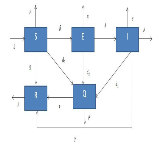
Figure 1.
Flowchart for the susceptible-exposed-infected-quarantine-recovered (SEIQR) epidemic model.
In this research article, we investigated a coronavirus (COVID-19) epidemic model with random perturbations, which was mainly constituted of five major classes: the susceptible population, the exposed class, the infected population, the quarantine class, and the population that has recovered. We studied the problem under consideration in order to derive at least one, and only one, nonlocal solution within the positive feasible region. The Lyapunov function was used to develop the necessary result of existence for ergodic stationary distribution and the conditions for the disease's extinction. According to our findings, the influence of Brownian motion and noise effects on epidemic transmission were powerful. The infection may diminish or eradicate if the noise is excessive. To illustrate our proposed scheme, we numerically simulated all classes' findings.
Citation: Rukhsar Ikram, Ghulam Hussain, Inayat Khan, Amir Khan, Gul Zaman, Aeshah A. Raezah. Stationary distribution of stochastic COVID-19 epidemic model with control strategies[J]. AIMS Mathematics, 2024, 9(11): 30413-30442. doi: 10.3934/math.20241468
| [1] | Jinji Du, Chuangliang Qin, Yuanxian Hui . Optimal control and analysis of a stochastic SEIR epidemic model with nonlinear incidence and treatment. AIMS Mathematics, 2024, 9(12): 33532-33550. doi: 10.3934/math.20241600 |
| [2] | Yue Wu, Shenglong Chen, Ge Zhang, Zhiming Li . Dynamic analysis of a stochastic vector-borne model with direct transmission and media coverage. AIMS Mathematics, 2024, 9(4): 9128-9151. doi: 10.3934/math.2024444 |
| [3] | Xiaodong Wang, Kai Wang, Zhidong Teng . Global dynamics and density function in a class of stochastic SVI epidemic models with Lévy jumps and nonlinear incidence. AIMS Mathematics, 2023, 8(2): 2829-2855. doi: 10.3934/math.2023148 |
| [4] | Yuhuai Zhang, Xinsheng Ma, Anwarud Din . Stationary distribution and extinction of a stochastic SEIQ epidemic model with a general incidence function and temporary immunity. AIMS Mathematics, 2021, 6(11): 12359-12378. doi: 10.3934/math.2021715 |
| [5] | Tingting Wang, Shulin Sun . Dynamics of a stochastic epidemic model with quarantine and non-monotone incidence. AIMS Mathematics, 2023, 8(6): 13241-13256. doi: 10.3934/math.2023669 |
| [6] | Ruoyun Lang, Yuanshun Tan, Yu Mu . Stationary distribution and extinction of a stochastic Alzheimer's disease model. AIMS Mathematics, 2023, 8(10): 23313-23335. doi: 10.3934/math.20231185 |
| [7] | Shah Hussain, Naveed Iqbal, Elissa Nadia Madi, Thoraya N. Alharthi, Ilyas Khan . Vaccination strategies in a stochastic $ \mathscr{SIVR} $ epidemic model. AIMS Mathematics, 2025, 10(2): 4441-4456. doi: 10.3934/math.2025204 |
| [8] | Yue Dong, Xinzhu Meng . Stochastic dynamic analysis of a chemostat model of intestinal microbes with migratory effect. AIMS Mathematics, 2023, 8(3): 6356-6374. doi: 10.3934/math.2023321 |
| [9] | Ruyue Hu, Chi Han, Yifan Wu, Xiaohui Ai . Analysis of a stochastic Leslie-Gower three-species food chain system with Holling-II functional response and Ornstein-Uhlenbeck process. AIMS Mathematics, 2024, 9(7): 18910-18928. doi: 10.3934/math.2024920 |
| [10] | Ying He, Bo Bi . Conditions for extinction and ergodicity of a stochastic Mycobacterium tuberculosis model with Markov switching. AIMS Mathematics, 2024, 9(11): 30686-30709. doi: 10.3934/math.20241482 |
In this research article, we investigated a coronavirus (COVID-19) epidemic model with random perturbations, which was mainly constituted of five major classes: the susceptible population, the exposed class, the infected population, the quarantine class, and the population that has recovered. We studied the problem under consideration in order to derive at least one, and only one, nonlocal solution within the positive feasible region. The Lyapunov function was used to develop the necessary result of existence for ergodic stationary distribution and the conditions for the disease's extinction. According to our findings, the influence of Brownian motion and noise effects on epidemic transmission were powerful. The infection may diminish or eradicate if the noise is excessive. To illustrate our proposed scheme, we numerically simulated all classes' findings.
Coronavirus SARS-CoV-2 (CoV-2) or the acute respiratory syndrome (SARS) is a respiratory virus. It's known as COVID-19 because of the virus that causes this disease (coronavirus disease 2019). COVID-19 was found in humans for the first time. During the middle of December, 2019, the epidemic was identified in the Chinese city of Wuhan in the province of Hubei. On January 30, 2020, the World Health Organization (WHO) stated that the SARS-CoV-2 outbreak had reached pandemic proportions and had been declared a global health emergency. Quarantine was put in place on January 23, 2020, by the Chinese government in Wuhan, China, to restrict the spread of the pandemic [1]. Mathematical modeling is a powerful technique for describing and dealing with diverse phenomena in nature. Recently, there has been a lot of focus on the development of mathematical models for understanding infectious diseases [2,3]. Many authors have established different epidemic models for the development and control of transmissible disease in communities. When compared to cardiovascular disease, infection-related diseases rank as the second leading cause of death on the globe. Mathematical models have become an important part of infectious disease epidemiology. In the twenty-first century, infectious diseases will become more prominent in both developed and developing countries. Global health challenges associated to infectious diseases are at an all-time high on the priority lists of world leaders, public health officials, and philanthropists, and they are expected to continue to rise in importance. Many researchers have spent the last few years using various ways to investigate infectious diseases and their mechanisms [4,5,6,7]. Aside from controlling the transmission of infectious diseases, this helps to prevent them in daily life. Epidemiological models are used to consider the advancement of contagious illnesses in populations. Many researchers have studied epidemic models to investigate and analyze diseases including avian influenza, hepatitis B, tuberculosis, and leishmaniasis [8,9,10]. We cannot use a single model to describe the entire disease system around the world since the existence or eradication of COVID-19 is dependent on so many different characteristics of the affected system. Since COVID-19, the human population has been quarantined, as the spread of the disease has been directly linked to this action. In most cases, quarantine is divided into two categories: One is infected whereas the other is susceptible quarantine. In this research work, we use the term "infected quarantine, " which refers to the practice of isolating those who have been exposed to an infectious disease and placing them in isolation.
Mathematical models have become an important part of infectious disease epidemiology. It has become popular to use mathematical modeling to study infectious illnesses that are communicable (see, for example, [11,12,13,14]). Mathematical modeling has been observed in the exploration of preventive mechanisms and propagations dynamics in recent years. Epidemiological models are used to take the spread of infectious diseases within the population into account [15,16]. One major area of concern for mathematical models in epidemiology is qualitative analysis. Deterministic and stochastic models distinguish between two categories of epidemic models. In comparison to its deterministic counterparts, the stochastic system is the most effective epidemic system for these forms and may even have a higher level of realism [17,18]. Because a stochastic model can be run multiple times to build up a distribution of the predicted results, as opposed to a deterministic model which can only yield a single predicted value, stochastic models yield more valuable results [19,20,21]. The stochastic nature of infectious disease transmission arises from the unpredictable nature of human contact.
Biological phenomena are often influenced by environmental noise in the real world. Beyond epidemiology, stochastic theory and techniques are widely used in other fields of nonlinear applied sciences. The stochastic approach has gained popularity due to its ability to accurately represent randomness and uncertainties in real-world scenarios. As a result, stochastic epidemic systems have been extensively studied (see [22]). Stochastic variations have long intrigued mathematicians and researchers because they can lead to significant changes that better align with real-world problems. For example, Rihan and Alsakaji [23] introduced a stochastic susceptible, infected, asymptomatic, quarantined, recovered (SIAQR) epidemic model for COVID-19 with time delays. In addition to qualitative analysis, they used reported data from the United Arab Emirates to predict the disease's behavior. Similarly, the authors in [24] proposed a stochastic susceptible-infected-recover-cross immune (SIRC) model for COVID-19, establishing sufficient conditions for the existence of an ergodic stationary distribution. They also showed that while diseases may go extinct under high levels of white noise, recurrence and periodic outbreaks are still possible due to the time-delayed feedback in transmission dynamics. The epidemic models can display qualitatively different dynamical behaviors when the conventional presumption of mass-action law is discarded. Numerous infectious illnesses like COVID-19 exhibit periodic changes in their prevalence. Such periodicities may be driven by extrinsic factors, as reflected in periodic transmission rates, e.g., seasonality [25], or may be caused by time delays (e.g., [26,27,28]) or nonlinearity of incidence rates. To describe the dynamics of COVID-19, the authors in [28] used the stochastic epidemic model with bilinear incidence rate and time-delay. In this study, we investigate the effects of weakening the bi-linearity assumption. As the disease COVID-19 is spreading at very fast rate with an increasing infected population, it is more realistic to consider the incidence of the form βSI(δI+1)N(t). Here, the notion N(t) is the total population which is further divided into five disjoint compartments, namely, vulnerable S(t), exposed E(t), infected I(t), quarantined Q(t), and recovered individuals R(t). To the best of our knowledge, in case of COVID-19, researchers have given less attention to the stochastic modeling with such type of incidence rates. Further, the authors discussed the qualitative analysis and controlling strategies that were completely ignored. Therefore, in this research work, we aim to prove the considerable effect of a stochastic factor on the dynamics and control of the COVID-19 epidemic model. Our model assumes that the total population is constant and that the parameters governing disease transmission and recovery are homogeneous across the entire population. This simplification may not accurately reflect real-world variations, such as changes in population behavior or differing rates of disease transmission across regions. The study relies on specific datasets for parameter estimation and model validation. These datasets are limited to certain regions and time frames, which may not capture all variations in disease dynamics. Consequently, the results may not be fully generalizable to other contexts or populations. While our model effectively captures the impact of stochastic noise on disease dynamics, it is sensitive to the choice of noise intensity parameters. Small changes in these parameters can lead to significantly different outcomes, which may pose challenges in real-world applications where precise parameter estimation is difficult. The stochastic nature of the model requires extensive computational resources for simulations, especially when exploring a wide range of noise intensities and control strategies. This may limit the model's applicability in scenarios where real-time analysis is required. The model and its conclusions are based on certain disease characteristics and may not be directly applicable to other infectious diseases with different transmission mechanisms or population structures. Further validation with different diseases and contexts is necessary to extend the findings.
Chen and Kang [29] presented a stochastic vaccination model with backward bifurcation and found that under some conditions, the smaller the intensity of the random perturbations is, the smaller the distance between the solution of the stochastic system and the stable equilibrium of the corresponding deterministic one. Cai et al. [30] discussed a stochastic susceptible-infected-recover (SIRS) epidemic model with nonlinear incidence rate and found stochastic perturbations can suppress the disease outbreak. Zhang et al. [31] presented a stochastic SIRS model with standard incidence rate and partial temporary immunity. Chang et al. [32] presented a stochastic SIRS epidemic model with two different saturated incidence rates and got the thresholds which leads to the extinction or persistence of the disease. These researches reveal that random fluctuations in the environment can restrain the spread of the disease. In other words, the transmission capacity of infectious diseases described by the deterministic model that ignores random perturbations is greater than their true transmission capacity. In this paper, our concern is when random fluctuations are introduced to the proposed system and whether they can also restrain the spread of the disease.
The paper is organized as follows. We developed the stochastic COVID-19 epidemic model in Section 2. The existence of global nonnegative solutions as well as an analysis of their uniqueness are examined in Section 3. Section 4 provides the necessary criteria for a stationary distribution to exist. In Section 5, we deduce conditions of extinction. Moreover, we discuss optimal control strategies in Section 6. To bolster our work in Section 7, numerical work in the form of simulations has been done. Finally, we wrapped up our work in Section 8.
To formulate the model, we will extend the model of Khan et al. [28] by incorporating the incidence rate of the form βSI(δI+1)N(t) and we will ignore the delay effect due to the fast spreading nature of the disease. We introduce noise as a stochastic term in our model, where it plays a critical role in capturing the random fluctuations in the system. In our normalized population model, the total population is scaled to unity, meaning that each subpopulation (e.g., susceptible, infected) represents a fraction of the total population. We define excessive noise as a level of stochastic fluctuation that becomes significant compared to the size of the subpopulations. Since the total population is normalized, noise that exceeds the corresponding subpopulation levels can cause unmanageable fluctuations, leading to dynamics that may no longer be reflective of the real-world scenarios the model aims to capture. For example, if the susceptible population constitutes 30% of the total population, noise levels approaching or exceeding this proportion would be deemed excessive. At this point, the noise introduces random fluctuations that overwhelm the deterministic trends in the model, potentially leading to unrealistic results. To capture the dynamics of COVID-19, we will use five ordinary differential equations and initially we formulate a deterministic mathematical model. The overall population is divided into five compartments i.e., S(t)+E(t)+I(t)+Q(t)+R(t)=N(t) with t as the independent variable. Following are the equations that illustrate the model:
| dSdt=b−βS(t)I(t)(δI(t)+1)N−(μ+d3+η)S(t),dEdt=βS(t)I(t)(δI(t)+1)N−(d2+λ+μ)E(t),dIdt=λE(t)−(ϵ+d1+μ+γ)I(t),dQdt=d2E(t)+d1I(t)+d3S(t)−(τ+μ)Q(t),dRdt=ηS(t)+γI(t)+τQ(t)−μR(t). | (2.1) |
The flow for this model is depicted in Figure 1. We assumed the incidence rate of the form βSI(δI+1)N because the infection COVID-19 spread too quickly as the infected population tends to increase. Here, the notion δ is a positive constant and biologically, it is a balance factor for the infected population. This incidence function could reduce the mass action law βSI if we set δ=0, which means the bilinear incidence rate is a special case of this function. To make the problem dimensionally homogenous, we must assume the unit per individual for the parameter δ. The description for the rest of the parameters are presented in Table 1.
| Notations | Descriptions | unit |
| b | The constant rate of birth | individualunittime |
| β | Coefficient of disease transmission rates | 1unittime |
| λ,τ,d1,d2,d3 | The state transition rates | 1unittime |
| ϵ | The rate at which people die due to the disease | 1unittime |
| μ | The natural mortality rate | 1unittime |
| δ | Balance factor for the infected individual | 1individual |
| η | The rate at which the susceptible class transmits to the recovered class | 1unittime |
| γ | The rate at which the infected individual moves to the recovered class | 1unittime |
 DownLoad:
CSV
DownLoad:
CSV
The stochastic form of the deterministic system (2.1) is represented as follows:
| dS(t)=[b−βS(t)I(t)(δI(t)+1)N−(d3+η+μ)S(t)]dt+α1SdW1(t),dE(t)=[βS(t)I(t)(δI(t)+1)N−(d2+λ+μ)E(t)]dt+α2EdW2(t),dI(t)=[λE(t)−(ϵ+d1+μ+γ)I(t)]dt+α3IdW3(t),dQ(t)=[d2E(t)+d1I(t)+d3S(t)−(μ+τ)Q]dt+α4QdW4(t),dR(t)=[ηS(t)+τQ(t)+γI(t)−μR]dt+α5RdW5(t). | (2.2) |
Here, Wi(t),i=1,...,5 are independent standard Brownian motions, and αi,i=1,...,5 are the intensities of the standard Gaussain white noises, respectively. The interaction between the environment and individuals are presented by α1SdW1(t),α2EdW2(t), and α3IdW3(t), α4QdW4(t), and α5RdW5(t).
In Section 3, we now emphasize that Theorem 2 establishes the existence and uniqueness of the solution to the stochastic differential equations that describe the model. Specifically, the theorem ensures that under the given assumptions, the stochastic system admits a unique stationary distribution, which implies long-term persistence or eradication of the disease, depending on the model parameters.
Additionally, we have clarified that the existence of the model refers to the mathematical formulation of the system, while existence and uniqueness of the solution refer to the behavior of the system over time under stochastic influences.
Theorem 1. There is a unique solution (S(t),E(t),I(t),Q(t),R(t)) of system (2.2) on t≥0 for any initial value ζ(0)=(S(0),E(0),I(0),Q(0),R(0))∈R5+., and the solution will remain in R5+ with probability one, namely, (S(t),E(t),I(t),Q(t),R(t))∈R5+ for all t≥0 almost surely.
Proof. For any ζ(0)∈R5+, the coefficients of our model accurately fulfill the Lipschitz local criterion. Consequently, ζ(t) represents a unique local solution for t∈[0,τe), where τe denotes the explosion time ([27]). We shall now demonstrate that the solution is still globally valid and establish τe=∞ a.s. When k0 is large enough to ensure that k0≥0, the starting approximation S(0), E(0), I(0), Q(0) and R(0) are in [1k0,k0]. We calculate the stopping time for k≥k0, as
| τk(τe)=inf{t∈[0,τe):max{S(t),E(t),I(t),Q(t),R(t)}≥kormin{S(t),E(t),I(t),Q(t),R(t))≤1k}}. | (3.1) |
In this study, we employ the concept of infϕ=∞, where ϕ represents null set, in accordance with the work of [33]. Since τk increases whenever k approaches to ∞, thus, limk→∞τk=τ∞ along the application of τ∞≤τe a.s showing that τ∞=∞ a.s. Accordingly, this will ensure the that solution of model (2.2) lies in R5+ a.s., ∀ 0≤t. To show that τe=∞ a.s, if this assertion is false, then there exist a pair of constants T>0 and ϵ∈(0,1) such that
| P{τ∞≤T}>ϵ. | (3.2) |
As a result, there is an integer k1≥k0 such that
| P{T≥τk}>ϵ,∀k1≤k. |
Consider a C2-mapping H:R5+→ˉR+, where ˉR+={x∈R:x≥0}, by
| H(S,E,I,Q,R)=(S−logS−1)+(E−logE−1)+(I−logI−1)+(Q−logQ−1)+(R−logR−1). | (3.3) |
Using the Itˆo′s formula in Eq (3.3) gives us
| dH(S,E,I,Q,R)=LH(S,E,I,Q,R)+α1(S−1)dW1(t)+α2(E−1)dW2(t)+α3(I−1)dW3(t)+α4(Q−1)dW4(t)+α5(R−1)dW5(t). | (3.4) |
The differential operator L associated to H in the above relation is given by
| L=∂∂t+(∂∂S,∂∂E,∂∂I,∂∂Q,∂∂R)⋅h(S,E,I,Q,R), |
where
| H(S,E,I,Q,R)=[b−βSI(δI+1)N−(d3+η+μ)S,βSI(δI+1)N−(d2+λ+μ)E,λE−(ϵ+d1+μ+γ)I,d2E+d1I(t)+d3S−(μ+τ)Q,γI+ηS+τQ(t)−μR]T. |
Thus in Eq (3.4), LH:R5+→R+, and we can write
| LH(S,E,I,Q,R)=(1−1S)(b−βSI(δI+1)N−(η+μ+d3)S)+α212+(1−1E)(βSI(δI+1)N−(d2+λ+μ)E)+α222+(1−1I)(λE−(μ+ϵ+γ+d1)I)+α232+(1−1Q)(d2E(t)+d1I+d3S−(μ+τ)Q)+α242+(1−1R)(γI+τQ+ηS−μR)+α252.LH(S,E,I,Q,R)=b−μ(S+E+I+Q+R)−ϵI−bS+βI(δI+1)N+(d3+η+μ)−βSI(δI+1)EN+(λ+μ+d2)−λEI+(μ+ϵ+γ+d1)−d2EQ−d3SQ−d1IQ+(τ+μ)−ηSR−τQR−γIR+α12+α22+α32+α42+α522≤b+β(1+δ)+η+5μ+d3+λ+d2+ϵ+γ+d1+τ+α12+α22+α32+α42+α522:=K. | (3.5) |
Since K is a positive constant therein independent of S,E,I,Q,R, and t, we can get
| dV(S,E,I,Q,R)≤Kdt+α1(S−1)dW1(t)+α2(E−1)dW2(t)+α3(I−1)dW3(t)+α4(Q−1)dW4(t)+α5(R−1)dW5(t). | (3.6) |
Integrating both sides (3.6) from 0 to T∧τk and taking expectations, we can obtain
| EH(S(τk),E(τk),I(τk),Q(τk),R(τk))≥H(S(0),E(0),I(0),Q(0),R(0))<∞, | (3.7) |
∀ k≥k1, assume T=Ωk & T≥τk, then P(Ωk)≥ϵ. Utilizing ω∈Ωk, for each, we find S(ω,τk), E(ω,τk), I(ω,τk), Q(ω,τk), R(ω,τk) values of which are based on k or 1k. Therefore, H(S(τk), E(τk,ω)), I(τk), Q(τk), R(τk) is not less than
| logk+1k−1orK−1−logk. |
Consequently,
| H(S(τk),E(τk),I(τk),Q(τk),R(τk))≥(logk+1k−1)∧(K−1−logk). | (3.8) |
From Eqs (3.7) and (3.8), we have
| KT+H(ζ(0))≥E[1Ω(ω)H(S(τk),E(τk),I(τk,Q(τk),R(τk)))]≥ϵ[(logk−1+1k)∧(K−1−logk)]. |
Here, 1Ω(ω) is used to represent the function indicator for Ωk. The contradiction develops when k approaches infinity, that is, ∞>H(S(0),E(0),I(0),Q(0),R(0)))+KT=∞, showing that τ∞=∞ a.s.
We investigate the system's proposed problem of stationary distribution (1). It really is easy to make a deterministic system by putting α1=α2=α3=α4=α5=0, the present version; on the other hand, is separate from its deterministic counterpart. Furthermore, we are aware that there is no endemic equilibrium in the stochastic system. Because of this, a linear stability analysis cannot be used to investigate the disease's permanence; instead, we look at the system's stationary distribution. Finally, this indicates that the illness will continue to exist. We shall use a well-known Khasminskii outcome for this [34]. Suppose
| 1t∫t0x(r)dr=⟨X(t)⟩, | (4.1) |
and for M=∫t0u(s)dB(s), we have
| ⟨M,M⟩t=∫t0(u(s))2ds. | (4.2) |
Lemma 1. By (Strong Law for large numbers)[35], if F={F}t≥0 is a real-valued continuous local martingale which goes away at t=0, then
| limt→∞⟨F,F⟩t=∞,⇒limt→∞Ft⟨F,F⟩t=0,a.s.and also,limt→∞sup⟨F,F⟩tt=0,⇒limt→∞Ftt=0,a.s. | (4.3) |
Different from the deterministic system (1.1), the stochastic system does not have the endemic equilibrium. Hence, we cannot study the persistence of the disease by studying their stability of the endemic equilibrium, and we turn to research the existence and uniqueness of the stationary distribution for the system (1.2) which implies the persistence of the disease in some sense. To this end, we cite a well-known result from Hasminskii [34]. Let X(t) be a regular time-homogeneous Markov process in Rn + described by
| b(X)dt+k∑rσrdWr(t)=dX(t). |
This is the display of the diffusion matrix:
| k∑r=1σir(x)σrj(x)=A(X)=(aij(x)),aij(x). |
Lemma 2. By [34], the unique stationary distribution m(⋅) of the Markov process X(t) is dependent upon the existence of a bounded domain U∈Rd with a regular boundary and its closure ¯U∈Rd, satisfying the following properties:
1) Within the open domain U and its surrounding areas, the diffusion matrix A(t)'s smallest eigenvalue is bounded away from zero.
2) If x∈RdU, then Supx∈kExτ<∞ for each compact subset K⊂Rn, and the time average "τ" at which a region originating from x goes to the finite set U. Furthermore, if f(.) is a function that can be integrated with respect to π, then
| ∫Rdf(x)π(dx))=1=P(limT→∞1T∫T0f(Xx(t))dt. |
Disease-free equilibrium in the deterministic model & the concerned stochastic system has a threshold value is given by
| Rd0=μβλ(d3+η+μ)(d2+λ+μ)(γ+μ+ϵ+d1). | (4.4) |
Following [36] and keeping in view the expression from Rd0, we can define a threshold parameter for the stochastic system of the form
| Rs0=μβλ(d3+η+μ+α212)(d2+λ+μ+α222)(γ+μ+ϵ+d1+α232). | (4.5) |
Theorem 2. If RS0>1, then the root (S(t),E(t),I(t),Q(t),R(t)) of model (2.2) is ergodic and there is only one stationary distribution π(.).
Proof. We demonstrate that, under condition (2) of Lemma 2, we need to construct a nonnegative C2−function V:R5+→R+. To this end, we first define
| V1=N+c1(−lnS)+c2(−lnE)+c3(−lnI), |
where it is necessary to identify the values of the three constants referred to in the problem, namely, c1, c2, and c3. We can calculate system (2.2) using Itô's formula.
| L(S+E+I+Q+R)=b−μ(N(t))−ϵI,L(−lnS)=−bS+βI(δI+1)N+(η+μ+d3)+α212,L(−lnE)=−βSI(δI+1)NE+λ+μ+d2+α222,L(−lnI)=−λEI+(μ+ϵ+γ+d1)+α232,L(−lnQ)=−d3SQ−d2EQ−d1IQ+(μ+τ)+α242,L(−lnR)=−ηSR−τQR−γIR+α252. | (4.6) |
Therefore, we have
| LV1=b−μ(S,E,I,Q,R)−ϵI−c1bS+c1βI(1+δI)N+c1(η+μ+d3)+c1α212−c2βSI(1+δI)NE+c2(λ+μ+d2)+c2α222−c3λEI+c3(μ+ϵ+γ+d1)+c3α232. |
The above implies that
| LV1≤−4[μ(N(t))×c1bS×c2βSI(N(t))E×c3λEI]14b−ϵI+c1βI(δI+1)N+c1(η+μ+d3)+α212)−c2βSI2NE+c2(λ+μ+d2+α222)+c3(μ+ϵ+γ+d1+α232). |
Let
| c1(d3+η+μ)+α212)=c2(d2+λ+μ+α222)=c3(μ+ϵ+γ+d1+α232)=b, |
namely,
| c1=b(d3+η+μ+α212),c2=b(d2+λ+μ+α222),c3=b(μ+ϵ+γ+d1+α232). | (4.7) |
Consequently,
| LV1≤−4[(b4μβλ(d3+η+μ+α212)(μ+λ+d2+α222)(μ+ϵ+γ+d1+α232))14−b]+c1βI(1+δI)N−c2βSI2NE−ϵI(t)LV1≤−4b[(RS0)1/4−1]+c1βI(δI+1)N. | (4.8) |
Furthermore, we acquire
| V2=c4(N+c2(−lnE)+c3(−lnI)+c1(−lnS))−(lnS+lnR+lnQ)+N(t)=(1+c4)(S+E+I+Q+R)−[lnR+c3c4lnI+lnQ+c2c4lnE+(1+c1c4)lnS], |
where c4>0 represents a constant to be determined later. It can be readily obtained that
| lim inf(S,E,I,Q,R)∈R5+∖UpV2(S,E,I,Q,R)=+∞,asp→∞, | (4.9) |
where (1p,p)×(1p,p)×(1p,p)=Up.
Following that, we will show that V2(S,E,I,Q,R) has unique minimum value V2(S0,E0,I0,Q0,R0). With respect to Q,R,I,S,E, the partial derivative of V2(S,E,I,Q,R) is as follows:
| ∂V2(S,E,I,Q,R)∂S=c4−1+c1c4S+1,∂V2(S,E,I,Q,R)∂E=−c2c4E+1+c4,∂V2(S,E,I,Q,R)∂I=1−c3c4I+c4,∂V2(S,E,I,Q,R)∂Q=−1Q+1+c4,∂V2(S,E,I,Q,R)∂R=1−1R+c4. |
It is easy to demonstrate that V2 has a only one stagnation point.
| (S(0),E(0),I(0),Q(0),R(0))=[(1+c1c41+c4,c2c4c4+1,c4c3c4+1,1c4+1,1c4+1)]. |
Furthermore, the Hessian matrix of V2(S,E,I,Q,R) at (S(0),E(0),I(0),Q(0),R(0)) is
| Λ=[1+c1c4S2(0)00000c2c4E2(0)00000c3c4I2(0)000001Q2(0)000001R2(0)]. |
This shows that Λ is obviously a nonnegative definite matrix. Therefore, V2(S,Q,E,I,R) has a minimum value V2(S0,E0,I0,Q0,R0).
According to Eq (4.9), and the continuity of V2(S,E,I,Q,R), we can conclude that in the interior of V2(S,E,I,Q,R) has a only one minimum value V2(S(0),E(0),I(0),Q(0),R(0)) belonging to R5+.
Moreover, we take into account a nonnegative C2− mapping V:R5+→R+ as follows:
| V(S,E,I,Q,R)=V2(S,E,I,Q,R)−V2(S(0),E(0),I(0),Q(0),R(0)). |
Ito's formula can be used to derive the proposed model.
| L(V)≤c4{−4b[−1+(˜RS0)1/4]+c1βI(δI+1)N}−bS+βI(δI+1)N+(η+μ+d3)+α212−d3SQ−d2EQ−d1IQ+(μ+τ)+α242−ηSR−τQR−γIR+α252+b−μN(t), | (4.10) |
the conclusion of which is as follows
| LV≤−c4c5+(c1c4+1)βI(δI+1)N−bS+βI(δI+1)N+(η+μ+d3)+α212−d3SQ−d2EQ−d1IQ+(μ+τ)+α242−ηSR−τQR−γIR+α252+b−μ(Q+E+S+I+R), | (4.11) |
where
| C5=4b[−1+(RS0)1/4]>0. |
The set Di represents a sequence of domains used to control the behavior of the solution and ensure it remains within a feasible region. The set Di is chosen based on the dynamics of the system to prevent the solution from approaching critical boundaries, such as zero or infinity. The following step is to define the set.
| D={ϵ1<S<1ϵ2,ϵ1<E<1ϵ2,ϵ1<I<1ϵ2,ϵ1<Q<1ϵ2,ϵ1<R<1ϵ2}, |
where εi>0(i=1,2,3,......10) indicate small constants that will be evaluated hereafter.
To investigate the convenience, R5+∖D can be divided into the ten domains listed below,
| D1={(S,E,I,Q,R)∈R5+,0<S≤ϵ1},D2={(S,E,I,Q,R)∈R5+,0<E≤ϵ1,S>ϵ2},D3={(S,E,I,Q,R)∈R5+,0<I≤ϵ1,E>ϵ2},D4={(S,E,I,Q,R)∈R5+,0<Q≤ϵ1,I>ϵ2},D5={(S,E,I,Q,R)∈R5+,0<R≤ϵ1,Q>ϵ2},D6={(S,E,I,Q,R)∈R5+,S≥1ϵ2},D7={(S,E,I,Q,R)∈R5+,E≥1ϵ2},D8={(S,E,I,Q,R)∈R5+,I≥1ϵ2},D9={(S,E,I,Q,R)∈R5+,Q≥1ϵ2},D10={(S,E,I,Q,R)∈R5+,R≥1ϵ2}. |
Next, we will demonstrate that LV(S,E,I,Q,R)<0 on R5+∖D using the same method from the ten domains mentioned above.
Case 1. According to Eq (4.11), if (S,E,I,Q,R)∈D1, we acquire
| LV≤−c4c5+(c1c4+1)βI(δI+1)N−bS+βI(δI+1)N+(η+μ+d3)+α212−d3SQ−d2EQ−d1IQ+(μ+τ)+α242−ηSR−τQR−γIR+α252+b−μN |
| ≤−c4c5+(c1c4+1)βI(δI+1)N−bϵ1+βI(δI+1)N+(η+μ+d3)+α212−d3SQ−d2EQ−d1IQ+(μ+τ)+α242−ηSR−τQR−γIR+α252+b−μN. |
Choosing ϵ1>0 yields
| LV<0whenever(S,E,I,Q,R)∈D1. | (4.12) |
Case 2. By Eq (4.11), if (S,E,I,Q,R)∈D2, we acquire
| LV≤−c4c5+(c1c4+1)βI(δI+1)N−bS+βI(δI+1)N+(η+μ+d3)+α212−d3SQ−d2EQ−d1IQ+(μ+τ)+α242−ηSR−τQR−γIR+α252+b−μN |
| ≤−c4c5+(c1c4+1)βI(δI+1)N−bS+βI(δI+1)N+(d3+η+μ)+α212−d3SQ−d2EQ−d1IQ+(μ+τ)+α242−ηSR−τQR−γIR+α252+b−μϵ2ϵ1. |
Let ϵ21=ϵ2. We can chose sufficiently enough large c4>0 and a small enough ϵ1>0 so that we can obtain
| LV<0whenever(S,E,I,Q,R)∈D2. | (4.13) |
Case 3. By Eq (4.11), if (S,E,I,Q,R)∈D3, we acquire
| LV≤−c4c5+(c1c4+1)βI(δI+1)N−bS+βI(δI+1)N+(η+μ+d3)+α212−d3SQ−d2EQ−d1IQ+(μ+τ)+α242−ηSR−τQR−γIR+α252+b−μN |
| ≤−c4c5+(c1c4+1)βI(δI+1)N−bS+βI(δI+1)N+(η+μ+d3)+α212−d3SQ−d2EQ−d1IQ+(μ+τ)+α242−ηSR−τQR−γIR+α252+b−μϵ1ϵ2. |
We can set a small enough ϵ1>0 so that we can obtain
| LV<0whenever(S,E,I,Q,R)∈D3. | (4.14) |
Case 4. By Eq (4.11), if (S,E,I,Q,R)∈D4, we acquire
| LV≤−c4c5+(c1c4+1)βI(δI+1)N−bS+βI(δI+1)N+(η+μ+d3)+α212−d3SQ−d2EQ−d1IQ+(μ+τ)+α242−ηSR−τQR−γIR+α252+b−μN |
| ≤−c4c5+(c1c4+1)βI(δI+1)N−bS+βI(δI+1)N+(η+μ+d3)+α212−d3SQ−d2EQ−d1ϵ2ϵ1+(μ+τ)+α242−ηSR−τQR−γIR+α252+b−μN. |
We can set a small enough ϵ2>0 so that we can obtain
| LV<0whenever(S,E,I,Q,R)∈D4. | (4.15) |
Case 5. According to Eq (4.11), if (S,E,I,Q,R)∈D5, we acquire
| LV≤−c4c5+(c1c4+1)βI(δI+1)N−bS+βI(δI+1)N+(η+μ+d3)+α212−d3SQ−d2EQ−d1IQ+(μ+τ)+α242−ηSR−τQR−γIR+α252+b−μN |
| ≤−c4c5+(c1c4+1)βI(δI+1)N−bS+βI(δI+1)N+(η+μ+d3)+α212−d3SQ−d2EQ−d1IQ+(μ+τ)+α242−ηSR−τϵ2ϵ1−γIR+α252+b−μN. |
We choose a small ϵ2>0 so that we can obtain
| LV<0whenever(S,E,I,Q,R)∈D5. | (4.16) |
Case 6. By Eq (4.11), if (S,E,I,Q,R)∈D6, we acquire
| LV≤−c4c5+(c1c4+1)βI(δI+1)N−bS+βI(δI+1)N+(η+μ+d3)+α212−d3SQ−d2EQ−d1IQ+(μ+τ)+α242−ηSR−τQR−γIR+α252+b−μN |
| −c4c5+(c1c4+1)βI(δI+1)N−bS+βI(δI+1)N+(η+μ+d3)+α212−d3SQ−d2EQ−d1IQ+(μ+τ)+α242−ηSR−τQR−γIR+α252+b−μϵ2. |
We may select a small enough ϵ2>0 so that we can obtain
| LV<0whenever(S,E,I,Q,R)∈D6. | (4.17) |
Case 7. By Eq (4.11), if (S,E,I,Q,R)∈D7, we acquire
| LV≤−c4c5+(c1c4+1)βI(δI+1)N−bS+βI(δI+1)N+(d3+η+μ)+α212−d3SQ−d2EQ−d1IQ+(μ+τ)+α242−ηSR−τQR−γIR+α252+b−μN |
| ≤−c4c5+(c1c4+1)βI(δI+1)N−bS+βI(δI+1)N+(d3+η+μ)+α212−d3SQ−d2EQ−d1IQ+(μ+τ)+α242−ηSR−τQR−γIR+α252+b−μϵ2. |
We choose a small ϵ2>0 so that we can obtain
| LV<0whenever(S,E,I,Q,R)∈D7. | (4.18) |
Case 8. If (S,E,I,Q,R)∈D8, from Eq (4.11), we have
| LV≤−c4c5+(c1c4+1)βI(δI+1)N−bS+βI(δI+1)N+(d3+η+μ)+α212−d3SQ−d2EQ−d1IQ+(μ+τ)+α242−ηSR−τQR−γIR+α252+b−μN |
| ≤−c4c5+(c1c4+1)βI(δI+1)N−bS+βI(δI+1)N+(d3+η+μ)+α212−d3SQ−d2EQ−d1IQ+(μ+τ)+α242−ηSR−τQR−γIR+α252+b−μϵ2. |
We can choose a small ϵ2>0 so that we can obtain
| LV<0whenever(S,E,I,Q,R)∈D8. | (4.19) |
Case 9. By Eq (4.11), if (S,E,I,Q,R)∈D9, we acquire
| LV≤−c4c5+(c1c4+1)βI(δI+1)N−bS+βI(δI+1)N+(η+μ+d3)+α212−d3SQ−d2EQ−d1IQ+(μ+τ)+α242−ηSR−τQR−γIR+α252+b−μN |
| ≤−c4c5+(c1c4+1)βI(δI+1)N−bS+βI(δI+1)N+(d3+η+μ)+α212−d3SQ−d2EQ−d1IQ+(μ+τ)+α242−ηSR−τQR−γIR+α252+b−μϵ2. |
If ϵ1>0, then we can find
| LV<0whenever(S,E,I,Q,R)∈D9. | (4.20) |
Case 10. If (S,E,I,Q,R)∈D10, from Eq (4.11), we have
| LV≤−c4c5+(c1c4+1)βI(δI+1)N−bS+βI(δI+1)N+(d3+η+μ)+α212−d2EQ−d3SQ−d1IQ+(μ+τ)+α242−ηSR−τQR−γIR+α252+b−μN |
| ≤−c4c5+(c1c4+1)βI(δI+1)N−bS+βI(δI+1)N+(η+μ+d3)+α212−d3SQ−d2EQ−d1IQ+(μ+τ)+α242−ηSR−τQR−γIR+α252+b−μϵ2. |
We can choose sufficiently small ϵ2>0 so we can obtain
| LV<0whenever(S,E,I,Q,R)∈D1. | (4.21) |
In conclusion, from 4.13 to 4.21, we can see that there exists a positive constant W>0 such that
| LV(S,E,I,Q,R)<−W<0for all(S,E,I,Q,R)∈R5+∖D. |
Hence,
| dV(S,E,I,Q,R)<[(1+c4)S−(1+c4c1)α1]dW1(t)+[(1+c4)E−c2c4α2]dW2(t)+[(1+c4)I−c3c4α3]dW3(t)+[(1+c4)Q−α4]dW4(t)+[(1+c4)R−α5]dW5(t)−Wdt. | (4.22) |
Let (S(0),E(0),I(0),Q(0),R(0))=(x1,x2,x3,x4,x5)=x∈R5+∖D, the time τx when a region originating from x approaches to D, min{τx,t,τk}=τ(k)(t), and τk=inf{tsuchthat|X|=k}.
| τk=inf{tsuchthat|X|=k}andτ(k)(t)=min{t,τk,τx}. |
Using Dynkins formula, we take expectation and integrate both sides of the Eq (4.22) from zero to τ(k)(t),
| EV(Q(τ(k)(t)),R(τ(k)(t)),I(τ(k)(t))−V(x)S(τ(k)(t)),E(τ(k)(t)))=E∫τ(k)(t)0LV(R(u),I(u),Q(u),E(u),S(u))du≤E∫τ(k)(t)0−Wdu=−WEτ(k)(t). |
Since V(x) is positive, hence
| V(x)W≥Eτ(k)(t). |
The proof of the outcome from Theorem 2 implies that P(τe=∞)=1. In other words, the system (2.2) is regular.
Therefore, we have that τ(k)(t) tends to τxalmost surely as k tends to ∞ and t→∞. As a result, with the assistance of Fatou's lemma, we arrive at
| ∞>V(x)W≥Eτ(n)(t). |
Obviously, supx∈KEτx<∞, where K denotes a compact subset of R5+. Consequently, condition (2) of Lemma 2 holds. Moreover, the model (2.2) diffusion matrix is provided by
| B=[α21S200000α22E200000α23I200000α24Q200000α25R2]. |
Consider M=min(S,E,I,Q,R)∈¯D∈R5+{σ21Q2,σ22E2,σ23I2,α24S2,α25R2}, and we have
| 5∑i,j=1aij(S,E,I,Q,R)ξiξj=α21S2ξ2+α22E2ξ22+α23I2ξ2+α24ξ24Q2+α25ξ25R2≥M|ξ|2,(Q,S,I,E,R)∈¯D, |
where ξi,i=1,2,3,4,5=ξ∈R5+.
By applying Lemma 2 and verifying that condition (1) of Lemma 2 holds, we have established that the diffusion matrix of the system is nondegenerate and bounded away from zero in the domain D. Furthermore, we have shown that the stopping time is τk→∞ as k→∞, ensuring that the system's solution remains in the positive region R5+ with probability one. Thus, conditions (1) and (2) of Lemma 2 are satisfied, implying the existence of a unique stationary distribution for the stochastic system. This stationary distribution reflects the long-term persistence of the disease within the population. Therefore, the statement of Theorem 2 is fully proved.
Concerning the disease's extinction, the following information is available to us.
Lemma 3. Assume a solution (s(t),E(t),I(t),Q(t),R(t)) of system (2.2) with starting condition (S(0),E(0),I(0),Q(0),R(0))∈R5+, then
| limt→∞(S(t),E(t),I(t),Q(t),R(t))<∞,a.s. |
Further, the root of the model has the following properties:
| {limt→∞S(t)t=:0,limt→∞E(t)t=:0,limt→∞I(t)t=:0,limt→∞Q(t)t=:0,limt→∞R(t)t=:0a.s., | (5.1) |
and
| {limt→∞lnS(t)t=0,limt→∞lnE(t)t=0,limt→∞lnI(t)t=0,limt→∞lnQ(t)t=0,limt→∞lnR(t)t=0a.s. | (5.2) |
Furthermore, when μ>12(α21∨α22∨α23∨α24∨α25) holds, then
| limt→∞1t∫t0S(r)dW1(r)=0,limt→∞1t∫t0E(r)dW2(r)=0,limt→∞1t∫t0I(r)dW3(r)=0,limt→∞1t∫t0Q(r)dW4(r)=0,limt→∞1t∫t0R(r)dW5(r)=0a.s. | (5.3) |
Proof. The proof follows the same approach as the proof of Lemma 4.1 in [37]. Therefore, we omit the details here.
Theorem 3. Let μ>(12)(α21∨α22∨α23∨α24∨α25), then (R(0),S(0),Q(0),I(0),E(0))∈R5+, and if
| ˜Rs0=2λβ(1+δ)(λ+μ+d2)(d2+μ+ϵ+γ+α232)(d2+λ+μ)2∧(λ2α222) | (5.4) |
holds, then
| limt→∞I(t)=0=limt→∞E(t)a.s. | (5.5) |
Moreover,
| limt→∞⟨S⟩=bη+μ+d3=S0,limt→∞⟨Q⟩=bd3(η+μ+d3)(μ+τ)=Q0,limt→∞⟨R⟩=b(η(μ+τ)+τd3)μ(η+μ+d3)(μ+τ)=R0a.s. | (5.6) |
Proof. Define a function W0, which is differentiable as follows:
| W0=ln[λE(t)+(λ+μ+d2)I(t)]. | (5.7) |
According to Ito's formula and model (2), we acquire
| dW0={λβSI(1+δI)N[λE(t)+(λ+μ+d2)I(t)]+(λ+μ+d2)(μ+ϵ+γ+d1)N[λE(t)+(λ+μ+d2)I(t)]−λ2α22E2+(λ+μ+d2)α23I22(λE(t)+(λ+μ+d2)I(t))2}dt+λα2EλE(t)+(λ+μ+d2)I(t)dW2+(λ+μ+d2)α3IλE(t)+(λ+μ+d2)I(t)dW3={λβ(1+δI)(λ+μ+d2)−(μ+ϵ+γ+d2+α232)(λ+μ+d2)2I2+(λ2α222E2)[λE(t)+(d2+λ+μ)I(t)]2}dt+λα2EλE(t)+(λ+μ+d2)I(t)dW2+(d2+λ+μ)α3IλE(t)+(d2+λ+μ)I(t)dW3={λβ(1+δ)(λ+μ+d2)−(μ+ϵ+γ+d2+α232)(λ+μ+d2)2∧(λ2α222)(λ+μ+d2)2}dt+λα2EλE(t)+(d2+λ+μ)I(t)dW2+(d2+λ+μ)α3IλE(t)+(d2+λ+μ)I(t)dW3. | (5.8) |
Divide by t on both sides of (5.8) and integrate from 0 to t. Also by Lemma 3, we have
| limsupt→∞ln[αE(t)+(α+μ)I(t)]t≤λβ(1+δ)(λ+μ+d2)−(μ+ϵ+γ+d2+α232)(λ+μ+d2)2∧(λ2α222)2(d2+λ+μ)2<0a.s., | (5.9) |
which illustrates that
| limt→∞I(t)=0=limt→∞E(t)a.s. | (5.10) |
Furthermore, the first equation of system (2) can be divided by t on both sides and integrated from zero to t to get a solution.
| S(t)−S(0)t=Π−β⟨SIN⟩−(ξ+μ)⟨S⟩+α1t∫t0S(r)dW1(r), | (5.11) |
which follows if we examine (5.10) and Lemma 3
| limt→∞⟨S⟩=bη+μ+d3=S0a.s. | (5.12) |
| limt→∞⟨Q⟩=bd3(η+μ+d3)(μ+τ)=Q0a.s. | (5.13) |
| limt→∞⟨R⟩=b(η(μ+τ)+τd3)μ(η+μ+d3)(μ+τ)=R0a.s. | (5.14) |
The proof for Theorem 3 has been completed.
Stochastic control of system (2) will take the same form as before, taking the same control variables into account.
| dS=[b−βSI(δI+1)N−(d3+η+μ+u1)S]dt+α1SdW1(t),dE=[βSI(δI+1)N−(d2+λ+μ)E]dt+α2EdW2(t),dI=[λE−(d1+μ+ϵ+γ+u2)I]dt+α3IdW3(t),dQ=[(u1+d3)S+(u2+d1)I+d2E−(μ+τ)Q]dt+α4QdW4(t),dR=[τQ+γI+ηS−μR]dt+α5RdW5(t). | (6.1) |
with the initial data
| S(0)>0,E(0)≥0,I(0)≥0,Q(0)≥0,R(0)>0. |
We establish a vector of the form for the purpose of simplicity.
| [z1,z2,z3,z4,z5]′=z(t),u(t)=[u2,u1]′, |
and
| dz(t)−g(z)dw(t)=f(z,u)dt, |
where the time functions zi and ui are used. It is also possible to represent the initial data in the form of
| z(0)=[z1,z2,z3,z4,z5]′(0)=z0. |
The following vector components are represented by the functions g and f.
| f1(x(t),u(t))=[b−βSI(δI+1)N−(d3+η+μ+u1)S]dt+α1SdW1(t),f2(x(t),u(t))=[(βSI(δI+1)N−(d2+μ+λ)E]dt+α2EdW2(t),f3(x(t),u(t))=[λE−(d1+μ+u2+ϵ+γ)I]dt+α3IdW3(t),f4(x(t),u(t))=[(u1+d3)S(t)+d2E(t)+(u2+d1)I−(τ+μ)Q]dt+α4QdW4(t),f5(x(t),u(t))=[γI+ηS+τQ−μR]dt+α5RdW5(t), | (6.2) |
g1=α1S,g2=α2E,g3=α3I,g4=α4Q,g5=α5R. In addition, we take into account the quadratic cost functional
| J(u)=12E{∫tf0(A1I+A2u21(t)2+A3u22(t)2)dt+k12S2+k22E2+k32I2k42Q2+k52R2}, |
where A1,A2,A3,kifori=1,2,...5 are nonnegative constants. In order to achieve our main objective, we must find a control u∗(t)=(u∗2(t),u∗1(t)) that allows us to perform this.
| J(u)≥J(u∗),foreveryu∈U. |
In this case, the set U denotes permissible controls.
| {uj(t):uj(t)∈[0,umaxj]=U,t∈(0,tf]∀uj∈L2[0,tf],wherej=1,2}. |
Here, umaxj, where j=1,2 is real and nonnegative. ˜Hamiltoniana for the given system must first be defined before the stochastic maximum principle can be applied to the system.
| G(z,u,m,n)=⟨g(z),n⟩−l(z,u)+⟨f(z,u),m⟩, | (6.3) |
where the inner product space of Euclidean is represented by ⟨.,.⟩ while the adjoint vectors systems [m1,m2,m3,m4,m5]′=m and [n1,n2,n3,n4,n5]′=n are different. The following is a direct expansion of the maximum principle
| −g(z∗(t))dW(t)+dz∗(t)=∂G(u∗,z∗,m,n)∂mdt. | (6.4) |
| −n(t)dW(t)+dm∗(t)=∂G(z∗,u∗,m,n)∂zdt. | (6.5) |
| minu∈UGm(z∗,u∗,m,n)=Gm(z∗,u∗,m,n), | (6.6) |
where z∗(t) represent the optimal path for z(t). The conditions for the start and end of Eqs (6.4) and (6.5) are
| z0=z∗(0) | (6.7) |
| −∂h(z∗(tf))∂z=m(tf), | (6.8) |
respectively. There is a mapping between "m(t), n(t), " and "z*(t)" in the optimal control, as shown in the Eq (6.6).
| u∗(t)=ϕ(z∗,m,n). | (6.9) |
As a result, the Hamiltonian in the given case is
| H=(A1I+A2u21(t)2+A3u22(t)2+k12S2+k22V2+k32E2k42I2+k52R2)+p1(b−βSI(δI+1)N−(η+μ+d3+u1)S)+p2(βSI(δI+1)N−(d2+λ+μ)E)+p3(λE−(d1+u2+μ+ϵ+γ)I)+p4((u1+d3)S+d2E(t)+(u2+d1)I−(τ+μ)Q)+p5(ηS+τQ+γI−μR)+α1Sq1+α2Eq2+α3Iq3+α4Qq4+α5Rq5. | (6.10) |
It is suggested by the stochastic maximum principle that
| −n(t)dW(t)+dm∗(t)=∂G(m,x∗,u∗,n)∂xdt. | (6.11) |
We obtain
| dm1dt=(m1(t)−m2(t))βI(δI+1)N+(d3+μ+u1(t)+η)m1(t)−(u1(t)+d3)m4(t)−ηm5+α1n1,dm2dt=m2(t)(d2+λ+μ)−m3(t)λ−d2m4(t)+α2n2,dm3dt=−A1+(m1(t)−m2(t))βS(1+δ)N+n3(t)(μ+ϵ+γ+d1+u2)−m4(u2+d1)−γm5+α3n3,dm4dt=m4(t)(μ+τ)−τp5(t)+α4n4,dm5dt=μm5(t)+α5n5. | (6.12) |
The auxiliary starting and ending criteria are also listed.
| S∗(0)=ˆS,E∗(0)=ˆE,I∗(0)=ˆI,Q∗(0)=ˆQ,R∗(0)=ˆR,m(tf)=−∂h(x∗(tf))∂x, | (6.13) |
and
| h(S,E,I,Q,R)=k12S2+k22E2+k32I2k42Q2+k52R2, | (6.14) |
where m1(tf)=−k1S,m2(tf)=−k2E,m3(tf)=−k3I,m4(tf)=−k4Q,m5(tf)=−k5R,. Now, by differentiating the Hamiltonian equation with respect to u1 and u2, we get the following optimal controls u∗1 and u∗2:
| max{min{1,1W1(m1−m4)S∗},0}=u∗1max{min{1,1W2(m3−m4)I∗},0}=u∗2. | (6.15) |
In the context of our stochastic modeling, we recognize the importance of providing a more comprehensive view of the inherent variability in our system. As such, we have incorporated confidence intervals in the figures to quantify the uncertainty around our estimates. Confidence intervals represent the range within which the system's state variables are expected to fluctuate due to the stochastic effects present in the model.
We will include a detailed explanation of how the level of noise is quantified relative to the sub-populations. Specifically:
● Low noise: Minor fluctuations that don't significantly affect the deterministic dynamics.
● Moderate noise: Fluctuations that introduce variability but still allow the population to follow predictable patterns over time.
● Excessive noise: Fluctuations on the same order of magnitude as the subpopulations (or higher), where random events can push the infected population toward extinction or cause erratic behavior.
For each simulated trajectory, we computed confidence intervals based on multiple realizations of the stochastic process. These intervals offer a visual representation of the range of potential outcomes, allowing for a better understanding of the variability in the disease dynamics. Specifically, 95% confidence intervals have been included in all figures to indicate the range in which the true values of the state variables lie, with 95% certainty.
Additionally, we have added stationary distributions to represent the long-term behavior of the system under stochastic influences. The stationary distribution reflects the equilibrium state that the system tends to settle into over time, despite random fluctuations. This distribution is crucial for understanding the persistent nature of the epidemic under stochastic dynamics.
The inclusion of both confidence intervals and stationary distributions enriches the analysis by highlighting the impact of stochasticity on the system's behavior, providing a clearer picture of both the short-term dynamics and the long-term tendencies of the epidemic model. In the following simulations, we consider three distinct cases to explore the different behaviors of the epidemic model under varying parameter settings. Each case corresponds to different combinations of the infection rate, recovery rate, and other model parameters:
● Case 1: Low infection rate and high recovery rate, simulating conditions leading to disease eradication.
● Case 2: Moderate infection rate and recovery rate, representing an endemic scenario where the disease persists.
● Case 3: High infection rate and low recovery rate, modeling a severe outbreak scenario.
These cases allow us to study the impact of different epidemiological factors on the dynamics of disease spread and control. Based on the deterministic SEIQR system, this stochastic system is a coupled system (2.1). Stochastic first order Runge Kutta approach is used to simulate numerical solution for system (2.2). Initially, in this section, we will show how to derive the stochastic Runge Kutta scheme for the system (2.2).
| Stn+1=Stn+[b−βNStnItn(1+δItn)−(η+μ+d3)Stn]Δtn+α1StnΔW1,tn+α21Stn((ΔW1,tn)2−Δtn)2√Δtn,Etn+1=Etn+[βNStnItn(1+δItn)−(λ+μ+d2)Etn]Δtn+α2tnΔW2,tn+α22Itn((ΔW2,tn)2−Δtn)2√Δtn,Itn+1=Itn+[λEtn−(μ+ϵ+γ+d1)Itn]Δtn+α3tnΔW3,tn+α23Itn((ΔW3,tn)2−Δtn)2√Δtn,Qtn+1=Qtn+[d3Stn+d2Etn+d1Itn−(μ+τ)Qtn]Δtb+α4QtnΔW4,tn+α24Qtn((ΔW4,tn)2−Δtn)2√Δtn,Rtn+1=Rtn+[ηStn+τQtn+γItn−μRtn]Δtn+α5RtndW5,tn+α25Rtn((ΔW5,tn)2−Δtn)2√Δtn. | (7.1) |
Here, ΔWi,tn=Wi,tn+1−Wi,tn, for i=1,...,5 represents the independent increments of the Gaussian Brownian motion and Δtn=tn+1−tn represents the time increment. In our case, we restrict ourself to a constant time step Δtn=Δt. 1000 equally spaced time increments are used to divide the interval. We numerically solve the SEIQR system (2) using the theoretical results shown above, with a number of randomly generated initial conditions. We run our code for generating three simulations. The first one is based on the choice of the parameter used in [28]. Similar choices of the parameter are used for the second and the third tests up to the parameter β. A list of the parameters that were used is provided in Table 2. For the mean solution, we generate 1000 realizations. The following correlation coefficients αi for i=1,2,...,5 with values in the range (0,1) are set for the three simulations by applying randomly chosen values to the uniform random generator. The following three scenarios are examined (see Table 2).
| Case 1 | Case 2 | Case 3 | |
| b | 0.028 | 0.028 | 0.028 |
| β | 0.5 | 0.25 | 0.25 |
| η | 0.6 | 0.6 | 0.6 |
| μ | 0.011 | 0.011 | 0.011 |
| λ | 0.3 | 0.3 | 0.3 |
| d1 | 0.2 | 0.2 | 0.1 |
| d2 | 0.08 | 0.08 | 0.08 |
| d3 | 0.06 | 0.06 | 0.06 |
| γ | 0.3 | 0.3 | 0.3 |
| τ | 0.1 | 0.1 | 0.1 |
| ϵ | 0.3 | 0.3 | 0.3 |
| α1 | 0.18246 | 0.21812 | 0.21812 |
| α2 | 0.02604 | 0.24036 | 0.24036 |
| α3 | 0.05651 | 0.01435 | 0.01435 |
| α4 | 0.10657 | 0.14235 | 0.14235 |
| α5 | 0.03730 | 0.22544 | 0.22544 |
| S0 | 0.14387 | 0.13228 | 0.13228 |
| Q0 | 0.27990 | 0.08732 | 0.08732 |
| I0 | 0.16027 | 0.27961 | 0.27961 |
| R0 | 0.27943 | 0.22923 | 0.22923 |
| E0 | 0.13645 | 0.27153 | 0.27153 |
DownLoad:
CSV
All of the individuals' initial values are chosen at random in the range of zero to one in the closed region [0,1]. For each step time, we establish the normatization
| 1=N(t),for everyt>0. |
It should be noted that model (2) operates based on five distinct independent white noises denoted as ΔWi(t) for i=1,2,...,5. The fourier series is being used to approximate the multiple stochastic integrals in order to assure the first order of our numerical approach [38].
Based on these values of parameters, we estimated both the parameters Rd0 and Rs0. It was obsreved that both the parameters are greater than one, therefore, the endemic equilibrium must exist in case of the deterministic model and the stochastic model should have a unique stationary distribution. To verify these facts numerically, we plotted Figures 2–4, which shows sample realizations of the stochastic SEIQR model (2.2). The corresponding mean solution is generated out of 1000 realizations. In the end, we concluded that outcomes in system (2.1) were satisfied by the simulations of Tests 1–3, namely, (S(t),E(t),I(t),Q(t),R(t))∈R5+ for some 0≤t. In addition, all SEIQR numerical stability has been verified in a series of tests (2.2). One can notice from the figures that the stochastic curves fluctuate around the endemic equilibrium, which in turns, shows the global stability of the endemic equilibrium of the associated deterministic system. Simulated trajectories of the infected population with 95% confidence intervals (shaded area) and corresponding stationary distribution, and simulated trajectories of the recovered population with 95% confidence intervals and stationary distribution are shown.


In this study, we have developed a novel stochastic epidemic model and demonstrated the existence of an ergodic stationary distribution, highlighting the role of noise in affecting disease dynamics. Unlike traditional deterministic models, our stochastic approach provides a more realistic representation of real-world uncertainties by capturing the randomness in disease transmission and recovery processes. This novel framework shows that noise can significantly influence the persistence of an epidemic and, in extreme cases, lead to extinction or recurrence of outbreaks. These findings contribute to the growing body of research on stochastic epidemic models, offering new perspectives on how randomness shapes epidemic outcomes.
Our study builds upon the extensive work done in epidemic modeling, particularly on the stochastic SEIR and SEIQR models. Previous works, such as those by Rihan and Alsakaji [23], Zhang et al. [31], and Cai et al. [30], introduced stochastic perturbations and nonlinear incidence rates to capture the uncertainties in disease transmission. However, these models often did not incorporate quarantine dynamics, which are crucial for COVID-19.
In contrast, our model extends this body of work by incorporating a quarantine class alongside stochastic perturbations driven by Brownian motion. The addition of quarantine in our SEIQR model provides a more realistic framework for understanding the feedback loop between noise intensity, infection rates, and quarantine measures. Similar to the findings by Zhang et al. [31], where stochastic noise could suppress disease spread, our results indicate that high noise levels can lead to disease extinction. However, our study goes further by illustrating the pivotal role of quarantine in this dynamic, which has not been explored in-depth in previous models.
By using the Lyapunov function, we also provide mathematical guarantees for the existence of ergodic stationary distributions, adding a layer of robustness to our results. This advances the field by offering more concrete tools for understanding the long-term behavior of epidemic systems under stochastic influences. Our findings suggest that noise and quarantine strategies, when properly managed, can significantly alter the trajectory of an epidemic, offering valuable insights for public health policymakers.
Future work: Moving forward, several extensions to this study can be explored. First, future work could investigate the impact of different types of noise, such as discrete-event noise or environmental fluctuations, which may offer a more accurate representation of real-world uncertainties. Additionally, the model could be expanded to consider heterogeneous populations or spatially structured networks, where the contact patterns between individuals vary based on factors like age, location, or social behavior. This would provide a more nuanced understanding of how epidemics spread in complex social systems.
Moreover, future research could focus on the transient dynamics of the model, particularly during the early stages of an outbreak, to better inform intervention strategies. Finally, validating the model with more case studies from different epidemic scenarios and diseases would enhance its applicability and robustness. By addressing these avenues in future work, the current model could be further refined to provide more comprehensive insights into epidemic dynamics under uncertainty.
R. Ikram: Formal analysis, Writing–original draft; G. Hussain: Validation, Software; I. Inayat: Resources, Software; A. Khan: Conceptualization, Supervision, Visualization, Methodology; G. Zaman: Data curation, Formal analysis; A. Raezah: Writing–review and editing, Investigation.
The authors extend their appreciation to the Deanship of Research and Graduate Studies at King Khalid University for funding this work through Research Group Project under grant number RGP 1/78/45.
The authors declare no conflict of interest.
| [1] |
C. C. Lai, T. P. Shih, W. C. Ko, H. J. Tang, P. R. Hsueh, Severe acute respiratory syndrome coronavirus 2 (SARS-CoV-2) and coronavirus disease-2019 (COVID-19): The epidemic and the challenges, Int. J. Antimicrob. Agents, 55 (2020), 105924. http://doi.org/10.1016/j.ijantimicag.2020.105924 doi: 10.1016/j.ijantimicag.2020.105924

|
| [2] |
R. J. de Groot, S. C. Baker, R. S. Baric, C. S. Brown, C. Drosten, L. Enjuanes, et al., Middle East respiratory syndrome coronavirus (MERS-CoV): Announcement of the Coronavirus Study Group, J. virol., 87 (2013), 7790–7792. http://doi.org/10.1128/JVI.01244-13 doi: 10.1128/JVI.01244-13
|
| [3] | The WHO MERS-CoV Research Group, State of knowledge and data gaps of Middle East respiratory syndrome coronavirus (MERS-CoV) in humans, PLoS Curr., 2013. |
| [4] | L. Arnold, Stochastic differential equations: Theory and applications, Wiley Interscience, 1974. |
| [5] |
Z. Wu, J. M. McGoogan, Characteristics of and important lessons from the coronavirus disease 2019 (COVID-19) outbreak in China: Summary of a report of 72314 cases from the Chinese Center for Disease Control and Prevention, JAMA, 323 (2020), 1239–1242. http://doi.org/10.1001/jama.2020.2648 doi: 10.1001/jama.2020.2648
|
| [6] |
A. Din, Y. Li, Q. Liu, Viral dynamics and control of hepatitis B virus (HBV) using an epidemic model, Alex. Eng. J., 59 (2020), 667–679. https://doi.org/10.1016/j.aej.2020.01.034 doi: 10.1016/j.aej.2020.01.034
|
| [7] |
A. Khan, G. Hussain, A. Yusuf, A. H. Usman, U. W. Humphries, A hepatitis stochastic epidemic model with acute and chronic stages, Adv. Differ. Equ., 2021 (2021), 181. https://doi.org/10.1186/s13662-021-03335-7 doi: 10.1186/s13662-021-03335-7
|
| [8] |
S. Qureshi, Z. Memon, Monotonically decreasing behavior of measles epidemic well captured by Atangana-Baleanu-Caputo fractional operator under real measles data of Pakistan, Chaos Soliton. Fract., 131 (2020), 109478. https://doi.org/10.1016/j.chaos.2019.109478 doi: 10.1016/j.chaos.2019.109478
|
| [9] |
T. Khan, A. Khan, G. Zaman, The extinction and persistence of the stochastic hepatitis B epidemic model, Chaos Soliton. Fract., 108 (2018), 123–128. https://doi.org/10.1016/j.chaos.2018.01.036 doi: 10.1016/j.chaos.2018.01.036
|
| [10] |
A. Gray, D. Greenhalgh, L. Hu, X. Mao, J. Pan, A stochastic differential equation SIS epidemic model, SIAM J. Appl. Math., 71 (2011), 876–902. https://doi.org/10.1137/10081856X doi: 10.1137/10081856X
|
| [11] |
G. Zaman, Y. H. Kang, I. H. Jung, Stability analysis and optimal vaccination of an SIR epidemic model, Biosystems, 93 (2008), 240–249. https://doi.org/10.1016/j.biosystems.2008.05.004 doi: 10.1016/j.biosystems.2008.05.004
|
| [12] |
L. Zou, W. Zhang, S. Ruan, Modeling the transmission dynamics and control of hepatitis B virus in China, J. Theor. Biol., 262 (2010), 330–338. https://doi.org/10.1016/j.jtbi.2009.09.035 doi: 10.1016/j.jtbi.2009.09.035
|
| [13] |
S. Thornley, C. Bullen, M. Roberts, Hepatitis B in a high prevalence New Zealand population: A mathematical model applied to infection control policy, J. Theor. Biol., 254 (2008), 599–603. https://doi.org/10.1016/j.jtbi.2008.06.022 doi: 10.1016/j.jtbi.2008.06.022
|
| [14] |
S. Zhao, Z. Xu, Y. Lu, A mathematical model of hepatitis B virus transmission and its application for vaccination strategy in China, Int. J. Epidemiol., 29 (2020), 744–752. https://doi.org/10.1093/ije/29.4.744 doi: 10.1093/ije/29.4.744
|
| [15] |
V. E. Papageorgiou, G. Vasiliadis, G. Tsaklidis, Analyzing the asymptotic behavior of an extended SEIR model with vaccination for COVID-19, Mathematics, 12 (2023), 55. https://doi.org/10.3390/math12010055 doi: 10.3390/math12010055
|
| [16] |
S. I. Araz, Analysis of a Covid-19 model: Optimal control, stability and simulations, Alex. Eng. J., 60 (2021), 647–658. https://doi.org/10.1016/j.aej.2020.09.058 doi: 10.1016/j.aej.2020.09.058
|
| [17] |
A. Mwasa, J. M. Tchuenche, Mathematical analysis of a cholera model with public health interventions, Biosystems, 105 (2011), 190–200. https://doi.org/10.1016/j.biosystems.2011.04.001 doi: 10.1016/j.biosystems.2011.04.001
|
| [18] |
Y. Zhou, W. Zhang, S. Yuan, Survival and stationary distribution of a SIR epidemic model with stochastic perturbations, Appl. Math. Comput., 244 (2014), 118–131. https://doi.org/10.1016/j.amc.2014.06.100 doi: 10.1016/j.amc.2014.06.100
|
| [19] |
V. E. Papageorgiou, Commentary on "Stochastic modeling of computer virus spreading with warning signals", J. Franklin I., 361 (2024), 106916. https://doi.org/10.1016/j.jfranklin.2024.106916 doi: 10.1016/j.jfranklin.2024.106916
|
| [20] |
J. R. Artalejo, M. J. Lopez-Herrero, Stochastic epidemic models: New behavioral indicators of the disease spreading, Appl. Math. Model., 38 (2014), 4371–4387. https://doi.org/10.1016/j.apm.2014.02.017 doi: 10.1016/j.apm.2014.02.017
|
| [21] |
G. Hussain, T. Khan, A. Khan, M. Inc, G. Zaman, K. S. Nisar, A. Akgül, Modeling the dynamics of novel coronavirus (COVID-19) via stochastic epidemic model, Alex. Eng. J., 60 (2021), 4121–4130. https://doi.org/10.1016/j.aej.2021.02.036 doi: 10.1016/j.aej.2021.02.036
|
| [22] | F. A. Rihan, H. J. Alsakaji, Analysis of a stochastic HBV infection model with delayed immune response, 18 (2021), 5194–5220. https://doi.org/10.3934/mbe.2021264 |
| [23] |
F. A. Rihan, H. J. Alsakaji, Dynamics of a stochastic delay differential model for COVID-19 infection with asymptomatic infected and interacting people: Case study in the UAE, Results Phys., 28 (2021), 104658. https://doi.org/10.1016/j.rinp.2021.104658 doi: 10.1016/j.rinp.2021.104658
|
| [24] |
F. A. Rihan, H. J. Alsakaji, C. Rajivganthi, Stochastic SIRC epidemic model with time-delay for COVID-19, Adv. Differ. Equ., 2020 (2020), 502. https://doi.org/10.1186/s13662-020-02964-8 doi: 10.1186/s13662-020-02964-8
|
| [25] |
W. P. London, J. A. Yorke, Recurrent outbreak of measles, chickenpox, and mumps. Ⅰ. Seasonal variation in contact rates, Am. J. Epidemiol., 98 (1973), 458–468. https://doi.org/10.1093/oxfordjournals.aje.a121575 doi: 10.1093/oxfordjournals.aje.a121575
|
| [26] | H. W. Hethcote, H. W. Stech, P. Van den Driessche, Nonlinear oscillations in epidemic models, SIAM J. Appl. Math., 40 (1981), 1–9. |
| [27] | X. Mao, Stochastic differential equations and their applications, Horwood, Chichester, 1997 |
| [28] |
A. Khan, R. Ikram, A. Din, U. W. Humphries, A. Akgul, Stochastic COVID-19 SEIQ epidemic model with time-delay, Results Phys., 30 (2021), 104775. https://doi.org/10.1016/j.rinp.2021.104775 doi: 10.1016/j.rinp.2021.104775
|
| [29] |
C. Chen, Y. Kang, The asymptotic behavior of a stochastic vaccination model with backward bifurcation, Appl. Math. Model., 40 (2016), 6051–6068. https://doi.org/10.1016/j.apm.2016.01.045 doi: 10.1016/j.apm.2016.01.045
|
| [30] |
Y. Cai, Y. Kang, W. Wang, A stochastic SIRS epidemic model with nonlinear incidence rate, Appl. Math. Comput., 305 (2017), 221–240. https://doi.org/10.1016/j.amc.2017.02.003 doi: 10.1016/j.amc.2017.02.003
|
| [31] |
X. B. Zhang, X. D. Wang, H. F. Huo, Extinction and stationary distribution of a stochastic SIRS epidemic model with standard incidence rate and partial immunity, Physica A, 531 (2019), 121548. https://doi.org/10.1016/j.physa.2019.121548 doi: 10.1016/j.physa.2019.121548
|
| [32] |
Z. Chang, X. Meng, X. Lu, Analysis of a novel stochastic SIRS epidemic model with two different saturated incidence rates, Physica A, 472 (2017), 103–116. https://doi.org/10.1016/j.physa.2017.01.015 doi: 10.1016/j.physa.2017.01.015
|
| [33] |
F. Wei, F. Chen, Stochastic permanence of an SIQS epidemic model with saturated incidence and independent random perturbations, Physica A, 453 (2016), 99–107. https://doi.org/10.1016/j.physa.2016.01.059 doi: 10.1016/j.physa.2016.01.059
|
| [34] | R. Khashminski, Stochastic stability of differential equations, Berlin: Springer-Verlag, 1980. |
| [35] |
C. Ji, D. Jiang, N. Shi, Multigroup SIR epidemic model with stochastic perturbation, Physica A, 390 (2011), 1747–1762. https://doi.org/10.1016/j.physa.2010.12.042 doi: 10.1016/j.physa.2010.12.042
|
| [36] |
A. Ríos-Gutiérrez, S. Torres, V. Arunachalam, Studies on the basic reproduction number in stochastic epidemic models with random perturbations, Adv. Differ. Equ., 2021 (2021), 288. https://doi.org/10.1186/s13662-021-03445-2 doi: 10.1186/s13662-021-03445-2
|
| [37] |
X. B. Zhang, X. D. Wang, H. F. Huo, Extinction and stationary distribution of a stochastic SIRS epidemic model with standard incidence rate and partial immunity, Physica A, 531 (2019), 121548. https://doi.org/10.1016/j.physa.2019.121548 doi: 10.1016/j.physa.2019.121548
|
| [38] |
M. Zahri, Multidimensional Milstein scheme for solving a stochastic model for prebiotic evolution, J. Taibah. Univ. Sci., 8 (2014), 186–198. https://doi.org/10.1016/j.jtusci.2013.12.002 doi: 10.1016/j.jtusci.2013.12.002
|
Figures(4) / Tables(2)

Rukhsar Ikram, Ghulam Hussain, Inayat Khan, Amir Khan, Gul Zaman, Aeshah A. Raezah. Stationary distribution of stochastic COVID-19 epidemic model with control strategies[J]. AIMS Mathematics, 2024, 9(11): 30413-30442. doi: 10.3934/math.20241468

| Notations | Descriptions | unit |
| b | The constant rate of birth | individualunittime |
| β | Coefficient of disease transmission rates | 1unittime |
| λ,τ,d1,d2,d3 | The state transition rates | 1unittime |
| ϵ | The rate at which people die due to the disease | 1unittime |
| μ | The natural mortality rate | 1unittime |
| δ | Balance factor for the infected individual | 1individual |
| η | The rate at which the susceptible class transmits to the recovered class | 1unittime |
| γ | The rate at which the infected individual moves to the recovered class | 1unittime |
DownLoad:
CSV
| Case 1 | Case 2 | Case 3 | |
| b | 0.028 | 0.028 | 0.028 |
| β | 0.5 | 0.25 | 0.25 |
| η | 0.6 | 0.6 | 0.6 |
| μ | 0.011 | 0.011 | 0.011 |
| λ | 0.3 | 0.3 | 0.3 |
| d1 | 0.2 | 0.2 | 0.1 |
| d2 | 0.08 | 0.08 | 0.08 |
| d3 | 0.06 | 0.06 | 0.06 |
| γ | 0.3 | 0.3 | 0.3 |
| τ | 0.1 | 0.1 | 0.1 |
| ϵ | 0.3 | 0.3 | 0.3 |
| α1 | 0.18246 | 0.21812 | 0.21812 |
| α2 | 0.02604 | 0.24036 | 0.24036 |
| α3 | 0.05651 | 0.01435 | 0.01435 |
| α4 | 0.10657 | 0.14235 | 0.14235 |
| α5 | 0.03730 | 0.22544 | 0.22544 |
| S0 | 0.14387 | 0.13228 | 0.13228 |
| Q0 | 0.27990 | 0.08732 | 0.08732 |
| I0 | 0.16027 | 0.27961 | 0.27961 |
| R0 | 0.27943 | 0.22923 | 0.22923 |
| E0 | 0.13645 | 0.27153 | 0.27153 |
DownLoad:
CSV
| Notations | Descriptions | unit |
| b | The constant rate of birth | individualunittime |
| β | Coefficient of disease transmission rates | 1unittime |
| λ,τ,d1,d2,d3 | The state transition rates | 1unittime |
| ϵ | The rate at which people die due to the disease | 1unittime |
| μ | The natural mortality rate | 1unittime |
| δ | Balance factor for the infected individual | 1individual |
| η | The rate at which the susceptible class transmits to the recovered class | 1unittime |
| γ | The rate at which the infected individual moves to the recovered class | 1unittime |
| Case 1 | Case 2 | Case 3 | |
| b | 0.028 | 0.028 | 0.028 |
| β | 0.5 | 0.25 | 0.25 |
| η | 0.6 | 0.6 | 0.6 |
| μ | 0.011 | 0.011 | 0.011 |
| λ | 0.3 | 0.3 | 0.3 |
| d1 | 0.2 | 0.2 | 0.1 |
| d2 | 0.08 | 0.08 | 0.08 |
| d3 | 0.06 | 0.06 | 0.06 |
| γ | 0.3 | 0.3 | 0.3 |
| τ | 0.1 | 0.1 | 0.1 |
| ϵ | 0.3 | 0.3 | 0.3 |
| α1 | 0.18246 | 0.21812 | 0.21812 |
| α2 | 0.02604 | 0.24036 | 0.24036 |
| α3 | 0.05651 | 0.01435 | 0.01435 |
| α4 | 0.10657 | 0.14235 | 0.14235 |
| α5 | 0.03730 | 0.22544 | 0.22544 |
| S0 | 0.14387 | 0.13228 | 0.13228 |
| Q0 | 0.27990 | 0.08732 | 0.08732 |
| I0 | 0.16027 | 0.27961 | 0.27961 |
| R0 | 0.27943 | 0.22923 | 0.22923 |
| E0 | 0.13645 | 0.27153 | 0.27153 |
