Comparison of two modified analytical approaches for the systems of time fractional partial differential equations

Aisha Abdullah Alderremy; Rasool Shah; Nehad Ali Shah; Shaban Aly; Kamsing Nonlaopon; Aisha Abdullah Alderremy; Rasool Shah; Nehad Ali Shah; Shaban Aly; Kamsing Nonlaopon

doi:10.3934/math.2023360

AIMS Mathematics

2023, Volume 8, Issue 3: 7142-7162. doi: 10.3934/math.2023360

Previous Article Next Article

Research article

Comparison of two modified analytical approaches for the systems of time fractional partial differential equations

1.
Department of Mathematics, Faculty of Science, King Khalid University, Abha 61413, Saudi Arabia
2.
Department of Mathematics, Abdul Wali Khan University, Mardan 23200, Pakistan
3.
Department of Mechanical Engineering, Sejong University, Seoul 05006, Korea
4.
Department of Mathematics, Faculty of Science, Al-Azhar University, Assiut 11884, Egypt
5.
Department of Mathematics, Faculty of Science, Khon Kaen University, Khon Kaen 40002, Thailand
† These authors contributed equally to this work and are co-first authors

Received: 12 August 2022 Revised: 24 November 2022 Accepted: 25 November 2022 Published: 11 January 2023
MSC : 33B15, 34A34, 35A20, 35A22, 44A10

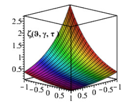
The aim of this article is to present a comparison of two analytical approaches toward obtaining the solution of the time-fractional system of partial differential equations. The newly proposed approaches are the new approximate analytical approach (NAAA) and Mohand variational iteration transform approach (MVITA). The NAAA is based on the Caputo-Riemann operator and its basic properties with the decomposition procedure. The NAAA provides step wise series form solutions with fractional order, which quickly converge to the exact solution for integer order. The MVITA is based on a variational iteration procedure and uses the Mohand integral transform. The MVITA also provides a series solution without a stepwise solution. Both approaches provide a series form of solutions to the proposed problems. The analytical procedures and obtained results are compared for the proposed problems. The obtained results were also compared with exact solutions for the problems. The obtained result and plots have shown the validity and applicability of the proposed algorithms. Both approaches can be extended for the analytical solution of other physical phenomena in science and technology.
Citation: Aisha Abdullah Alderremy, Rasool Shah, Nehad Ali Shah, Shaban Aly, Kamsing Nonlaopon. Comparison of two modified analytical approaches for the systems of time fractional partial differential equations[J]. AIMS Mathematics, 2023, 8(3): 7142-7162. doi: 10.3934/math.2023360

Related Papers:

Abstract

The aim of this article is to present a comparison of two analytical approaches toward obtaining the solution of the time-fractional system of partial differential equations. The newly proposed approaches are the new approximate analytical approach (NAAA) and Mohand variational iteration transform approach (MVITA). The NAAA is based on the Caputo-Riemann operator and its basic properties with the decomposition procedure. The NAAA provides step wise series form solutions with fractional order, which quickly converge to the exact solution for integer order. The MVITA is based on a variational iteration procedure and uses the Mohand integral transform. The MVITA also provides a series solution without a stepwise solution. Both approaches provide a series form of solutions to the proposed problems. The analytical procedures and obtained results are compared for the proposed problems. The obtained results were also compared with exact solutions for the problems. The obtained result and plots have shown the validity and applicability of the proposed algorithms. Both approaches can be extended for the analytical solution of other physical phenomena in science and technology.

References

[1]	J. H. He, Homotopy perturbation technique, Comput. Methods Appl. Mech. Eng., 178 (1999), 257–262. https://doi.org/10.1016/S0045-7825(99)00018-3 doi: 10.1016/S0045-7825(99)00018-3
[2]	X. J. Wu, D. R. Lai, H. T. Lu, Generalized synchronization of the fractional-order chaos in weighted complex dynamical networks with nonidentical nodes, Nonlinear Dynam., 69 (2012), 667–683. https://doi.org/10.1007/s11071-011-0295-9 doi: 10.1007/s11071-011-0295-9
[3]	H. Sheng, Y. Q. Chen, T. S. Qiu, Fractional Processes and Fractional-Order Signal Processing, London: Springer, 2011. https://doi.org/10.1007/978-1-4471-2233-3
[4]	H. Nasrolahpour, A note on fractional electrodynamics, Commun. Nonlinear Sci., 18 (2013), 2589–2593. https://doi.org/10.1016/j.cnsns.2013.01.005 doi: 10.1016/j.cnsns.2013.01.005
[5]	P. Veeresha, D. G. Prakasha, H. M. Baskonus, New numerical surfaces to the mathematical model of cancer chemotherapy effect in Caputo fractional derivatives, Chaos An Interdiscip. J. Nonlinear Sci., 29 (2019), 013119. https://doi.org/10.1063/1.5074099 doi: 10.1063/1.5074099
[6]	S. Longhi, Fractional Schrodinger equation in optics, Opt. lett., 40 (2015), 1117–1120. https://doi.org/10.1364/OL.40.001117 doi: 10.1364/OL.40.001117
[7]	S. Ullah, M. A. Khan, M. Farooq, A new fractional model for the dynamics of the hepatitis B virus using the Caputo-Fabrizio derivative, Eur. Phys. J. Plus, 133 (2018), 237. https://doi.org/10.1140/epjp/i2018-12072-4 doi: 10.1140/epjp/i2018-12072-4
[8]	M. A. Khan, S. Ullah, M. Farooq, A new fractional model for tuberculosis with relapse uia Atangana-Baleanu deriuatiue, Chaos Soliton Fract., 116 (2018), 227–238. https://doi.org/10.1016/j.chaos.2018.09.039 doi: 10.1016/j.chaos.2018.09.039
[9]	M. A. Khan, S. Ullah, K. O. Okosun, K. Shah, A fractional order pine wilt disease model with Caputo-Fabrizio deriuatiue, Adv. Differ. Equ., 2018 (2018), 410. https://doi.org/10.1186/s13662-018-1868-4 doi: 10.1186/s13662-018-1868-4
[10]	J. Singh, D. Kumar, D. Baleanu, On the analysis of fractional diabetes model with exponential law, Adv. Differ. Equ., 2018 (2018), 231. https://doi.org/10.1186/s13662-018-1680-1 doi: 10.1186/s13662-018-1680-1
[11]	R. Hilfer, Applications of Fractional Calculus in Physics, 2000. https://doi.org/10.1142/3779
[12]	A. A. Kilbas, H. M. Srivastava, J. J. Trujillo, Theory and Applications of Fractional Differential Equations, Amsterdam, Boston: Elsevier, 2006.
[13]	S. Das, A note on fractional diffusion equations, Chaos Soliton Fract., 42 (2009), 2074–2079. https://doi.org/10.1016/j.chaos.2009.03.163 doi: 10.1016/j.chaos.2009.03.163
[14]	R. Ye, P. Liu, K. B. Shi, B. Yan, State damping control: A novel simple method of rotor UAV with high performance, IEEE Access, 8 (2020), 214346–214357. https://doi.org/10.1109/ACCESS.2020.3040779 doi: 10.1109/ACCESS.2020.3040779
[15]	K. Liu, Z. X. Yang, W. F. Wei, B. Gao, D. L. Xin, C. M. Sun, et al., Novel detection approach for thermal defects: Study on its feasibility and application to vehicle cables, High Volt., 2022, 1–10. https://doi.org/10.1049/hve2.12258 doi: 10.1049/hve2.12258
[16]	P. Liu, J. P. Shi, Z. A. Wang, Pattern formation of the attraction-repulsion Keller-Segel system, Discrete Continuous Dyn. Syst. B, 18 (2013), 2597–2625. https://doi.org/10.3934/dcdsb.2013.18.2597 doi: 10.3934/dcdsb.2013.18.2597
[17]	J. G. Liu, X. J. Yang, J. J. Wang, A new perspective to discuss Korteweg-de Vries-like equation, Phys. Lett. A, 451 (2022), 128429. https://doi.org/10.1016/j.physleta.2022.128429 doi: 10.1016/j.physleta.2022.128429
[18]	Z. H. Xie, X. A. Feng, X. J. Chen, Partial least trimmed squares regression, Chemometr. Intell. Lab. Syst., 221 (2022), 104486. https://doi.org/10.1016/j.chemolab.2021.104486 doi: 10.1016/j.chemolab.2021.104486
[19]	Z. T. Shao, Q. Z. Zhai, Z. H. Han, X. H. Guan, A linear AC unit commitment formulation: An application of data-driven linear power flow model, Int. J. Elec. Power, 145 (2023), 108673. https://doi.org/10.1016/j.ijepes.2022.108673 doi: 10.1016/j.ijepes.2022.108673
[20]	V. N. Kovalnogov, R.V. Fedorov, T. V. Karpukhina, T. E. Simos, C. Tsitouras, Runge-Kutta pairs of orders 5(4) trained to best address keplerian type orbits, Mathematics, 9 (2021), 2400. https://doi.org/10.3390/math9192400 doi: 10.3390/math9192400
[21]	N. A. Shah, H. A. Alyousef, S. A. El-Tantawy, J. D. Chung, Analytical investigation of fractional-order Korteweg-De-Vries-type equations under Atangana-Baleanu-Caputo operator: Modeling nonlinear waves in a plasma and fluid, Symmetry, 14 (2022), 739. https://doi.org/10.3390/sym14040739 doi: 10.3390/sym14040739
[22]	R. Shah, H. Khan, D. Baleanu, P. Kumam, M. Arif, The analytical investigation of time-fractional multi-dimensional Navier-Stokes equation, Alex. Eng. J., 59 (2020), 2941–2956. https://doi.org/10.1016/j.aej.2020.03.029 doi: 10.1016/j.aej.2020.03.029
[23]	K. Nonlaopon, M. Naeem, A. M. Zidan, R. Shah, A. Alsanad, A. Gumaei, Numerical investigation of the time-fractional Whitham-Broer-Kaup equation involving without singular kernel operators, Complexity, 2021 (2021), 7979365. https://doi.org/10.1155/2021/7979365 doi: 10.1155/2021/7979365
[24]	S. Alyobi, A. Khan, N. A. Shah, K. Nonlaopon, Fractional analysis of nonlinear boussinesq equation under Atangana-Baleanu-Caputo operator, Symmetry, 14 (2022), 2417. https://doi.org/10.3390/sym14112417 doi: 10.3390/sym14112417
[25]	S. Mukhtar, S. Noor, The numerical investigation of a fractional-order multi-dimensional model of Navier-Stokes equation via novel techniques, Symmetry, 14 (2022), 1102. https://doi.org/10.3390/sym14061102 doi: 10.3390/sym14061102
[26]	V. B. L. Chaurasia, D. Kumar, Solution of the time-fractional Navier-Stokes equation, Gen. Math. Notes, 4 (2011), 49–59.
[27]	A. Prakash, P. Veeresha, D. G. Prakasha, M. Goyal, A new efficient technique for solving fractional coupled Navier–Stokes equations using q-homotopy analysis transform method, Pramana, 93 (2019), 6. https://doi.org/10.1007/s12043-019-1763-x doi: 10.1007/s12043-019-1763-x
[28]	A. A. Alderremy, N. A. Shah, S. Aly, K. Nonlaopon, Evaluation of fractional-order pantograph delay differential equation via modified laguerre wavelet method, Symmetry, 14 (2022), 2356. https://doi.org/10.3390/sym14112356 doi: 10.3390/sym14112356
[29]	H. Thabet, S. Kendre, J. Peters, Travelling wave solutions for fractional Korteweg-de Vries equations via an approximate-analytical method, AIMS Mathematics, 4 (2019), 1203–1222. https://doi.org/10.3934/math.2019.4.1203 doi: 10.3934/math.2019.4.1203
[30]	B. R. Sontakke, A. S. Shaikh, Properties of Caputo operator and its applications to linear fractional differential equations, Int. J. Eng. Res. Appl., 5 (2015), 22–27.
[31]	S. Momani, Z. Odibat, Analytical solution of a time-fractional Navier–Stokes equation by Adomian decomposition method, Appl. Math. Comput., 177 (2006), 488–494. https://doi.org/10.1016/j.amc.2005.11.025 doi: 10.1016/j.amc.2005.11.025
[32]	N. A. Shah, Y. S. Hamed, K. M. Abualnaja, J. D. Chung, A. Khan, A comparative analysis of fractional-order kaup-kupershmidt equation within different operators, Symmetry, 14 (2022), 986. https://doi.org/10.3390/sym14050986 doi: 10.3390/sym14050986
[33]	M. M. Al-Sawalha, O. Y. Ababneh, K. Nonlaopon, Numerical analysis of fractional-order Whitham-Broer-Kaup equations with non-singular kernel operators, AIMS Mathematics, 8 (2023), 2308–2336. https://doi.org/10.3934/math.2023120 doi: 10.3934/math.2023120
[34]	T. Botmart, R. P. Agarwal, M. Naeem, A. Khan, R. Shah, On the solution of fractional modified Boussinesq and approximate long wave equations with non-singular kernel operators, AIMS Mathematics, 7 (2022), 12483–12513. https://doi.org/10.3934/math.2022693 doi: 10.3934/math.2022693
[35]	D. Kumar, J. Singh, A. Prakash, R. Swroop, Numerical simulation for system of time-fractional linear and nonlinear differential equations, Prog. Fract. Differ. Appl., 5 (2019), 65–77. https://doi.org/10.18576/pfda/050107 doi: 10.18576/pfda/050107
[36]	M. Goyal, H. M. Baskonus, A. Prakash, An efficient technique for a time fractional model of lassa hemorrhagic fever spreading in pregnant women, Eur. Phys. J. Plus, 134 (2019), 482. https://doi.org/10.1140/epjp/i2019-12854-0 doi: 10.1140/epjp/i2019-12854-0
[37]	H. M. He, J. G. Peng, H. Y. Li, Iterative approximation of fixed point problems and variational inequality problems on Hadamard manifolds, UPB Sci. Bull. Series A, 84 (2022), 25–36.
[38]	L. Liu, L. Zhang, G. Pan, S. Zhang, Robust yaw control of autonomous underwater vehicle based on fractional-order PID controller, Ocean Eng., 257 (2022), 111493. https://doi.org/10.1016/j.oceaneng.2022.111493 doi: 10.1016/j.oceaneng.2022.111493
[39]	A. Prakash, H. Kaur, Analysis and numerical simulation of fractional Biswas-Milovic model, Math. Comput. Simulat., 181 (2021), 298–315. https://doi.org/10.1016/j.matcom.2020.09.016 doi: 10.1016/j.matcom.2020.09.016
[40]	A. Prakash, M. Goyal, S. Gupta, A reliable algorithm for fractional Bloch model arising in magnetic resonance imaging, Pramana, 92 (2019), 18. https://doi.org/10.1007/s12043-018-1683-1 doi: 10.1007/s12043-018-1683-1
[41]	M. Goyal, H. M. Baskonus, A. Prakash, Regarding new positive, bounded and convergent numerical solution of nonlinear time fractional HIV/AIDS transmission model, Chaos Soliton Fract., 139 (2020), 110096. https://doi.org/10.1016/j.chaos.2020.110096 doi: 10.1016/j.chaos.2020.110096

Reader Comments

Your name:*

Email:*
© 2023 the Author(s), licensee AIMS Press. This is an open access article distributed under the terms of the Creative Commons Attribution License (http://creativecommons.org/licenses/by/4.0)