Simulation analysis, properties and applications on a new Burr XII model based on the Bell-X functionalities

Ayed. R. A. Alanzi; Muhammad Imran; M. H. Tahir; Christophe Chesneau; Farrukh Jamal; Saima Shakoor; Waqas Sami; Ayed. R. A. Alanzi; Muhammad Imran; M. H. Tahir; Christophe Chesneau; Farrukh Jamal; Saima Shakoor; Waqas Sami

doi:10.3934/math.2023352

AIMS Mathematics

2023, Volume 8, Issue 3: 6970-7004. doi: 10.3934/math.2023352

Previous Article Next Article

Research article

Simulation analysis, properties and applications on a new Burr XII model based on the Bell-X functionalities

1.
Department of Mathematics, College of Science and Arts, Jouf University, Gurayat, Saudi Arabia
2.
Department of Statistics, The Islamia University of Bahawalpur, Punjab 63100, Pakistan
3.
Université de Caen Normandie, LMNO, Campus II, Science 3, Caen 14032, France
4.
Department of Mathematics, The Islamia University of Bahawalpur, Bahawalpur, Pakistan
5.
College of Nursing, QU Health, Qatar University, Doha, P.O. Box 2713, Qatar

Received: 02 December 2022 Revised: 21 December 2022 Accepted: 02 January 2023 Published: 11 January 2023
MSC : 60E05, 62N05, 62F10, 62D05

In this article, we make mathematical and practical contributions to the Bell-X family of absolutely continuous distributions. As a main member of this family, a special distribution extending the modeling perspectives of the famous Burr XII (BXII) distribution is discussed in detail. It is called the Bell-Burr XII (BBXII) distribution. It stands apart from the other extended BXII distributions because of its flexibility in terms of functional shapes. On the theoretical side, a linear representation of the probability density function and the ordinary and incomplete moments are among the key properties studied in depth. Some commonly used entropy measures, namely Rényi, Havrda and Charvat, Arimoto, and Tsallis entropy, are derived. On the practical (inferential) side, the associated parameters are estimated using seven different frequentist estimation methods, namely the methods of maximum likelihood estimation, percentile estimation, least squares estimation, weighted least squares estimation, Cramér von-Mises estimation, Anderson-Darling estimation, and right-tail Anderson-Darling estimation. A simulation study utilizing all these methods is offered to highlight their effectiveness. Subsequently, the BBXII model is successfully used in comparisons with other comparable models to analyze data on patients with acute bone cancer and arthritis pain. A group acceptance sampling plan for truncated life tests is also proposed when an item's lifetime follows a BBXII distribution. Convincing results are obtained.
- Burr XII distribution,
- entropy measures,
- estimation,
- GASP,
- quality parameter,
- T-X family
Citation: Ayed. R. A. Alanzi, Muhammad Imran, M. H. Tahir, Christophe Chesneau, Farrukh Jamal, Saima Shakoor, Waqas Sami. Simulation analysis, properties and applications on a new Burr XII model based on the Bell-X functionalities[J]. AIMS Mathematics, 2023, 8(3): 6970-7004. doi: 10.3934/math.2023352

Related Papers:

Abstract

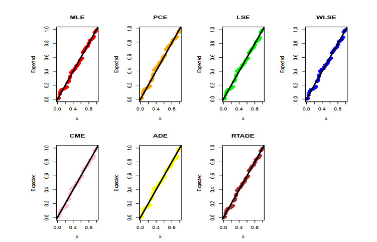
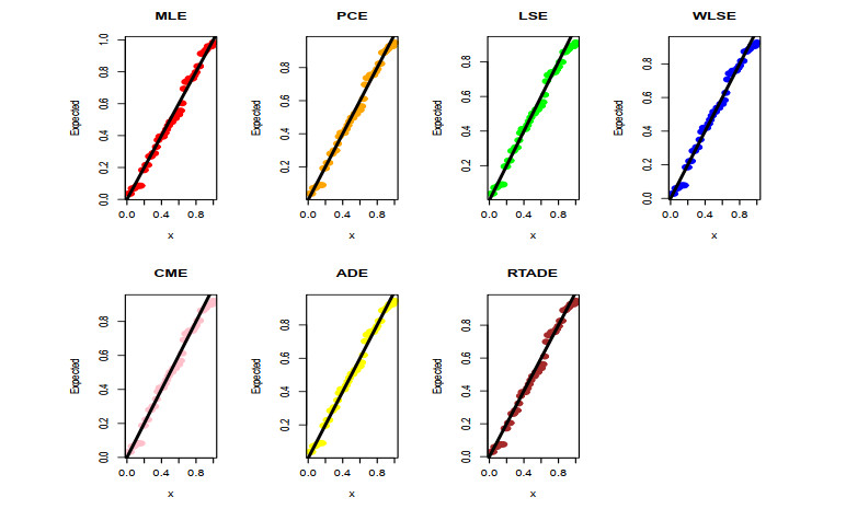
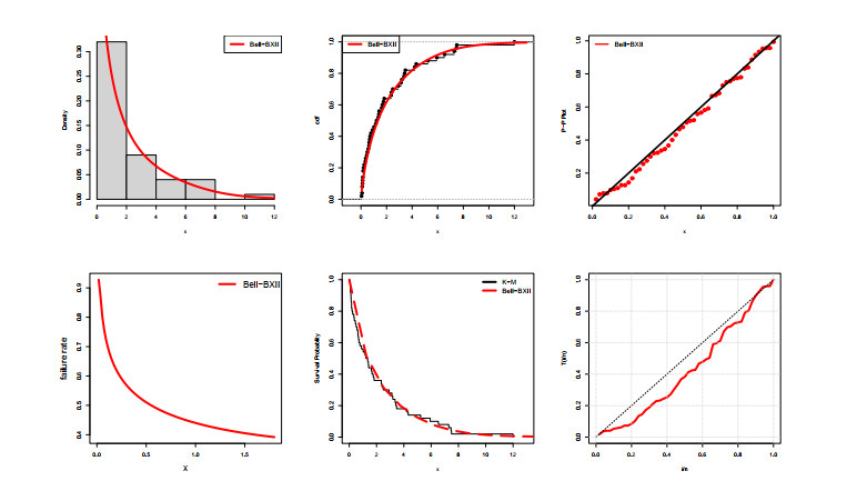
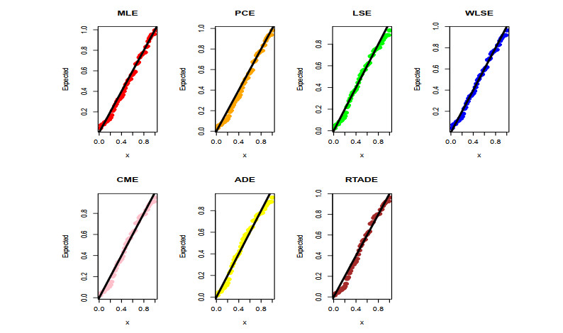
In this article, we make mathematical and practical contributions to the Bell-X family of absolutely continuous distributions. As a main member of this family, a special distribution extending the modeling perspectives of the famous Burr XII (BXII) distribution is discussed in detail. It is called the Bell-Burr XII (BBXII) distribution. It stands apart from the other extended BXII distributions because of its flexibility in terms of functional shapes. On the theoretical side, a linear representation of the probability density function and the ordinary and incomplete moments are among the key properties studied in depth. Some commonly used entropy measures, namely Rényi, Havrda and Charvat, Arimoto, and Tsallis entropy, are derived. On the practical (inferential) side, the associated parameters are estimated using seven different frequentist estimation methods, namely the methods of maximum likelihood estimation, percentile estimation, least squares estimation, weighted least squares estimation, Cramér von-Mises estimation, Anderson-Darling estimation, and right-tail Anderson-Darling estimation. A simulation study utilizing all these methods is offered to highlight their effectiveness. Subsequently, the BBXII model is successfully used in comparisons with other comparable models to analyze data on patients with acute bone cancer and arthritis pain. A group acceptance sampling plan for truncated life tests is also proposed when an item's lifetime follows a BBXII distribution. Convincing results are obtained.

References

[1]	C. Lee, F. Famoye, A. Y. Alzaatreh, Methods for generating families of univariate continuous distributions in the recent decades, Wiley Interdiscip. Rev.: Comput. Stat., 5 (2013), 219–238. https://doi.org/10.1002/wics.1255 doi: 10.1002/wics.1255
[2]	S. K. Maurya, S. Nadarajah, Poisson generated family of distributions: a review, Sankhya B, 83 (2021), 484–540. https://doi.org/10.1007/s13571-020-00237-8 doi: 10.1007/s13571-020-00237-8
[3]	M. H. Tahir, G. M. Cordeiro, Compounding of distributions: a survey and new generalized classes, J. Stat. Distrib. Appl., 3 (2016), 13. https://doi.org/10.1186/s40488-016-0052-1 doi: 10.1186/s40488-016-0052-1
[4]	A. Alzaatreh, C. Lee, F. Famoye, A new method for generating families of continuous distributions, METRON, 71 (2013), 63–79. https://doi.org/10.1007/s40300-013-0007-y doi: 10.1007/s40300-013-0007-y
[5]	I. W. Burr, Cumulative frequency functions, Ann. Math. Stat., 13 (1942), 215–232.
[6]	R. N. Rodriguez, A guide to the Burr type XII distributions, Biometrika, 64 (1977), 129–134. https://doi.org/10.1093/biomet/64.1.129 doi: 10.1093/biomet/64.1.129
[7]	R. V. da Silva, F. Gomes-Silva, M. W. A. Ramos, G. M. Cordeiro, The exponentiated Burr XII Poisson distribution with application to lifetime data, Int. J. Stat. Probab., 4 (2015), 112. https://doi.org/10.5539/ijsp.v4n4p112 doi: 10.5539/ijsp.v4n4p112
[8]	P. F. Paranaíba, E. M. Ortega, G. M. Cordeiro, M. A. de Pascoa, The Kumaraswamy Burr XII distribution: theory and practice, J. Stat. Comput. Simul., 83 (2013), 2117–2143. https://doi.org/10.1080/00949655.2012.683003 doi: 10.1080/00949655.2012.683003
[9]	A. Y. Al-Saiari, L. A. Baharith, S. A. Mousa, Marshall-Olkin extended Burr type XII distribution, Int. J. Stat. Probab., 3 (2014), 78–84. https://doi.org/10.5539/ijsp.v3n1p78 doi: 10.5539/ijsp.v3n1p78
[10]	H. M. Reyad, S. A. Othman, The Topp-Leone Burr-XII distribution: properties and applications, Br. J. Math. Comput. Sci., 21 (2017), 1–15.
[11]	P. F. Paranaíba, E. M. M. Ortega, G. M. Cordeiro, R. R. Pescim, The beta Burr XII distribution with application to lifetime data, Comput. Stat. Data Anal., 55 (2011), 1118–1136. https://doi.org/10.1016/j.csda.2010.09.009 doi: 10.1016/j.csda.2010.09.009
[12]	W. J. Zimmer, J. B. Keats, F. K. Wang, The Burr XII distribution in reliability analysis, J. Qual. Technol., 30 (1998), 386–394. https://doi.org/10.1080/00224065.1998.11979874 doi: 10.1080/00224065.1998.11979874
[13]	P. R. Tadikamalla, A look at the Burr and related distributions, Int. Stat. Review/Revue Int. Stat., 48 (1980), 337–344. https://doi.org/10.2307/1402945 doi: 10.2307/1402945
[14]	C. Kleiber, S. Kotz, Statistical size distributions in economics and actuarial sciences, John Wiley & Sons, 2003. https://doi.org/10.1002/0471457175
[15]	E. T. Bell, Exponential polynomials, Ann. Math., 35 (1934), 258–277. https://doi.org/10.2307/1968431
[16]	F. Castellares, S. L. P. Ferrari, A. J. Lemonte, On the Bell distribution and its associated regression model for count data, Appl. Math. Model., 56 (2018), 172–185. https://doi.org/10.1016/j.apm.2017.12.014 doi: 10.1016/j.apm.2017.12.014
[17]	A. Fayomi, M. Tahir, A. Algarni, M. Imran, F. Jamal, A new useful exponential model with applications to quality control and actuarial data, Comput. Intel. Neurosci., 2022 (2022), 2489998. https://doi.org/10.1155/2022/2489998 doi: 10.1155/2022/2489998
[18]	M. H. Tahir, M. Zubair, G. M. Cordeiro, A. Alzaatreh, M. Mansoor, The Poisson-X family of distributions, J. Stat. Comput. Simul., 86 (2016), 2901–2921. https://doi.org/10.1080/00949655.2016.1138224 doi: 10.1080/00949655.2016.1138224
[19]	A. Z. Afify, O. A. Mohamed, A new three-parameter exponential distribution with variable shapes for the hazard rate: estimation and applications, Mathematics, 8 (2020), 135. https://doi.org/10.3390/math8010135 doi: 10.3390/math8010135
[20]	M. Nassar, A. Z. Afify, M. K. Shakhatreh, S. Dey, On a new extension of Weibull distribution: properties, estimation, and applications to one and two causes of failures, Qual. Reliab. Eng. Int., 36 (2020), 2019–2043. https://doi.org/10.1002/qre.2671 doi: 10.1002/qre.2671
[21]	T. Dey, D. Kundu, Two-parameter Rayleigh distribution: different methods of estimation, Amer. J. Math. Manage. Sci., 33 (2014), 55–74. https://doi.org/10.1080/01966324.2013.878676 doi: 10.1080/01966324.2013.878676
[22]	S. Dey, S. Ali, C. Park, Weighted exponential distribution: properties and different methods of estimation, J. Stat. Comput. Simul., 85 (2015), 3641–3661. https://doi.org/10.1080/00949655.2014.992346 doi: 10.1080/00949655.2014.992346
[23]	S. Dey, T. Dey, S. Ali, M. S. Mulekar, Two-parameter Maxwell distribution: properties and different methods of estimation, J. Stat. Theory Pract., 10 (2016), 291–310. https://doi.org/10.1080/15598608.2015.1135090 doi: 10.1080/15598608.2015.1135090
[24]	S. Dey, A. Alzaatreh, C. Zhang, D. Kumar, A new extension of generalized exponential distribution with application to ozone data, Ozone: Sci. Eng., 39 (2017), 273–285. https://doi.org/10.1080/01919512.2017.1308817 doi: 10.1080/01919512.2017.1308817
[25]	J. H. Kao, Computer methods for estimating Weibull parameters in reliability studies, IRE T. Reliab. Qual. Control, PGRQC-13 (1958), 15–22. https://doi.org/10.1109/IRE-PGRQC.1958.5007164 doi: 10.1109/IRE-PGRQC.1958.5007164
[26]	J. M. Amigó, S. G. Balogh, S. Hernández, A brief review of generalized entropies, Entropy, 20 (2018), 813. https://doi.org/10.3390/e20110813 doi: 10.3390/e20110813
[27]	S. H. Abid, U. J. Quaez, J. E. Contreras-Reyes, An information-theoretic approach for multivariate skew-t distributions and applications, Mathematics, 9 (2021), 146. https://doi.org/10.3390/math9020146 doi: 10.3390/math9020146
[28]	C. G. Small, Expansions and asymptotics for statistics, 1 Ed., Chapman and Hall/CRC, 2010. https://doi.org/10.1201/9781420011029
[29]	J. J. Swain, S. Venkatraman, J. R. Wilson, Least-squares estimation of distribution functions in Johnson's translation system, J. Stat. Comput. Simul., 29 (1988), 271–297. https://doi.org/10.1080/00949658808811068 doi: 10.1080/00949658808811068
[30]	P. Macdonald, Comments and queries comment on "An estimation procedure for mixtures of distributions" by Choi and Bulgren, J. Royal Stat. Soc.: Ser. B (Methodol.), 33 (1971), 326–329. https://doi.org/10.1111/j.2517-6161.1971.tb00884.x doi: 10.1111/j.2517-6161.1971.tb00884.x
[31]	T. W. Anderson, D. A. Darling, Asymptotic theory of certain "goodness of fit" criteria based on stochastic processes, Ann. Math. Stat., 23 (1952), 193–212. https://doi.org/10.1214/aoms/1177729437 doi: 10.1214/aoms/1177729437
[32]	M. Mansour, H. M. Yousof, W. Shehata, M. Ibrahim, A new two parameter Burr XII distribution: properties, copula, different estimation methods and modeling acute bone cancer data, J. Nonlinear Sci. Appl., 13 (2020), 223-238. http://dx.doi.org/10.22436/jnsa.013.05.01 doi: 10.22436/jnsa.013.05.01
[33]	H. M. Okasha, M. Shrahili, A new extended Burr XII distribution with applications, J. Comput. Theor. Nanosci., 14 (2017), 5261–5269. https://doi.org/10.1166/jctn.2017.6930 doi: 10.1166/jctn.2017.6930
[34]	A. M. Almarashi, K. Khan, C. Chesneau, F. Jamal, Group acceptance sampling plan using Marshall-Olkin Kumaraswamy exponential (MOKw-E) distribution, Processes, 9 (2021), 1066. https://doi.org/10.3390/pr9061066 doi: 10.3390/pr9061066
[35]	C. H. Jun, S. Balamurali, S. H. Lee, Variables sampling plans for Weibull distributed lifetimes under sudden death testing, IEEE T. Reliab., 55 (2006), 53–58. https://doi.org/10.1109/TR.2005.863802 doi: 10.1109/TR.2005.863802
[36]	C. W. Wu, W. L. Pearn, A variables sampling plan based on Cpmk for product acceptance determination, Eur. J. Oper. Res., 184 (2008), 549–560. https://doi.org/10.1016/j.ejor.2006.11.032 doi: 10.1016/j.ejor.2006.11.032
[37]	J. Chen, S. T. B. Choy, K. H. Li, Optimal Bayesian sampling acceptance plan with random censoring, Eur. J. Oper. Res., 155 (2004), 683–694. https://doi.org/10.1016/S0377-2217(02)00889-5 doi: 10.1016/S0377-2217(02)00889-5
[38]	A. J. Fernández, Progressively censored variables sampling plans for two-parameter exponential distributions, J. Appl. Stat., 32 (2005), 823–829. https://doi.org/10.1080/02664760500080074 doi: 10.1080/02664760500080074
[39]	W. L. Pearn, C. W. Wu, Variables sampling plans with PPM fraction of defectives and process loss consideration, J. Oper. Res. Soc., 57 (2006), 450–459. https://doi.org/10.1057/palgrave.jors.2602013 doi: 10.1057/palgrave.jors.2602013
[40]	A. J. Fernández, C. J. Pérez-González, M. Aslam, C. H. Jun, Design of progressively censored group sampling plans for Weibull distributions: an optimization problem, Eur. J. Oper. Res., 211 (2011), 525–532. https://doi.org/10.1016/j.ejor.2010.12.002 doi: 10.1016/j.ejor.2010.12.002

Reader Comments

Your name:*

Email:*
© 2023 the Author(s), licensee AIMS Press. This is an open access article distributed under the terms of the Creative Commons Attribution License (http://creativecommons.org/licenses/by/4.0)