A special class of triple starlike trees characterized by Laplacian spectrum

Muhammad Ajmal; Xiwang Cao; Muhammad Salman; Jia-Bao Liu; Masood Ur Rehman; Muhammad Ajmal; Xiwang Cao; Muhammad Salman; Jia-Bao Liu; Masood Ur Rehman

doi:10.3934/math.2021260

AIMS Mathematics

2021, Volume 6, Issue 5: 4394-4403. doi: 10.3934/math.2021260

Previous Article Next Article

Research article

A special class of triple starlike trees characterized by Laplacian spectrum

1.
Department of Mathematics, Nanjing Univesity of Aeronautics and Astronautics, Nanjing, Jiangsu 211100, P. R. China
2.
Department of Mathematics, The Islamia University of Bahawalpur, Bahawalpur 63100, Pakistan
3.
School of Mathematics and Physics, Anhui Jianzhu University, Hefei, Anhui 230601, P. R. China
4.
Department of Basic Sciences, Balochistan University of Engineering and Technology Khuzdar, Khuzdar 89100, Pakistan

Received: 24 December 2020 Accepted: 04 February 2021 Published: 20 February 2021
MSC : 05C50

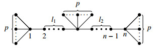
Two graphs are said to be cospectral with respect to the Laplacian matrix if they have the same Laplacian spectrum. A graph is said to be determined by the Laplacian spectrum if there is no other non-isomorphic graph with the same Laplacian spectrum. In this paper, we prove that one special class of triple starlike tree is determined by its Laplacian spectrum.
- Laplacian spectrum,
- tree,
- triple starlike tree
Citation: Muhammad Ajmal, Xiwang Cao, Muhammad Salman, Jia-Bao Liu, Masood Ur Rehman. A special class of triple starlike trees characterized by Laplacian spectrum[J]. AIMS Mathematics, 2021, 6(5): 4394-4403. doi: 10.3934/math.2021260

Related Papers:

Abstract

Two graphs are said to be cospectral with respect to the Laplacian matrix if they have the same Laplacian spectrum. A graph is said to be determined by the Laplacian spectrum if there is no other non-isomorphic graph with the same Laplacian spectrum. In this paper, we prove that one special class of triple starlike tree is determined by its Laplacian spectrum.

References

[1]	R. Boulet, B. Jouve, The lollipop is determined by its spectrum, Electron. J. Comb., 15 (2008), R74. doi: 10.37236/798
[2]	R. Boulet, Spectral characterizations of sun graphs and broken sun graphs, Discrete Math. Theor. Comput. Sci., 11 (2009), 149–160.
[3]	C. J. Bu, J. Zhou, Starlike trees whose maximum degree exceed 4 are determined by their Q-spectra, Linear Algebra Appl., 436 (2012), 143–151. doi: 10.1016/j.laa.2011.06.028
[4]	C. J. Bu, J. Zhou, Signless Laplacian spectral characterization of the cones over some regular graphs, Linear Algebra Appl., 436 (2012), 3634–3641. doi: 10.1016/j.laa.2011.12.035
[5]	N. Ghareghani, G. R. Omidi, B. Tayfeh-Rezaie, Spectral characterization of graphs with index at most $\sqrt{2+\sqrt{5}}$, Linear Algebra Appl., 420 (2007), 483–489. doi: 10.1016/j.laa.2006.08.009
[6]	Hs. H. Günthard, H. Primas, Zusammenhang von Graphentheorie und Mo-Theorie von Molekeln mit Systemen konjugierter Bindungen, Helv. Chim. Acta., 39 (1956), 1645–1653. doi: 10.1002/hlca.19560390623
[7]	I. Gutman, V. Gineityte, M. Lepović, M. Petrović, The high-energy band in the photoelectron spectrum of alkaners and its dependence on molecular structure, J. Serb. Chem. Soc., 64 (1999), 673–680. doi: 10.2298/JSC9911673G
[8]	A. K. Kelmans, V. M. Chelnokov, A certain polynomial of a graph and graphs with an extremal number of trees, J. Comb. Theory B, 16 (1974), 197–214. doi: 10.1016/0095-8956(74)90065-3
[9]	D. J. Klein, Graph geometry, graph metrics, & wiener, MATCH Communi. Math. Compt. Chem., 35 (1997), 7–27.
[10]	J. X. Li, X. D. Zhang, On the Laplacian eigenvalues of a graph, Linear Algebra Appl., 285 (1998), 305–307. doi: 10.1016/S0024-3795(98)10149-0
[11]	X. G. Liu, Y. P. Zhang, P. L. Lu, One special double starlike graph is determined by its Laplacian spectrum, Appl. Math. Lett., 22 (2009), 435–438. doi: 10.1016/j.aml.2008.06.012
[12]	F. J. Liu, Q. X. Huang, Laplacian spectral characterization of 3-rosegraphs, Linear Algebra Appl., 439 (2013), 2914–2920. doi: 10.1016/j.laa.2013.07.029
[13]	M. L. Liu, Y. L. Zhu, H. Y. Shan, K. C. Das, The spectral characterization of butterfly-like graphs, Linear Algebra Appl., 513 (2017), 55–68. doi: 10.1016/j.laa.2016.10.003
[14]	P. L. Lu, X. D. Zhang, Y. P. Zhang, Determination of double quasi-star tree from its Laplacian spectrum, Journal Shanghai University, 14 (2010), 163–166. doi: 10.1007/s11741-010-0622-1
[15]	P. L. Lu, X. G. Liu, Laplacian spectral characterization of some double starlike trees, Journal of Harbin Engineering University, 37 (2016), 242–247.
[16]	X. L. Ma, Q. X. Huang, Signless Laplacian spectral characterization of 4-rose graphs, Linear Multi-linear Algebra, 64 (2016), 2474–2485. doi: 10.1080/03081087.2016.1161705
[17]	M. Mirzakhah, D. Kiani, The sun graph is determined by its signless Laplacian spectrum, Electron. J. Linear Algebra, 20 (2010), 610–620.
[18]	G. R. Omidi, K. Tajbakhsh, Startlike trees are determined by their Laplacian spectrum, Linear Algebra Appl., 422 (2007), 654–658. doi: 10.1016/j.laa.2006.11.028
[19]	C. S. Oliveira, N. M. M. de Abreu, S. Jurkiewicz, The characteristic polynomial of the Laplacian of graphs in $(a, b)$-linear cases, Linear Algebra Appl., 356 (2002), 113–121. doi: 10.1016/S0024-3795(02)00357-9
[20]	G. R. Omidi, E. Vatandoost, Starlike trees with maximum degree 4 are determined by their signless Laplacian spectra, Electron. J. Linear Algebra, 20 (2010), 274–290.
[21]	X. L. Shen, Y. P. Hou, Y. P. Zhang, Graph $ Z_n $ and some graphs related to $ Z_n $ are determined by their spectrum, Linear Algebra Appl., 404 (2005), 58–68. doi: 10.1016/j.laa.2005.01.036
[22]	X. L. Shen, Y. P. Hou, Some trees are determined by their Laplacian spectra, Journal of Nature Science Hunan Normal University, 1 (2006), 241–272.
[23]	S. Sorgun, H. Topcu, On the spectral characterization of kite graphs, J. Algebra Comb. Discrete Struct. Appl., 3 (2016), 81–90.
[24]	E. R. van Dam, W. H. Haemers, Which graphs are determined by their spectrum? Linear Algebra Appl., 373 (2003), 241–272.
[25]	E. R. van Dam, W. H. Haemers, Developments on spectral characterizations of graphs, Discrete Math., 309 (2009), 576–586. doi: 10.1016/j.disc.2008.08.019
[26]	W. Wang, C. X. Xu, Note: The T-shape tree is determined by its Laplacian spectrum, Linear Algebra Appl., 419 (2006), 78–81. doi: 10.1016/j.laa.2006.04.005
[27]	F. Wen, Q. X. Huang, X. Y. Huang, F. J. Liu, On the Laplacian spectral characterization of $\prod$-shape trees, Indian J. Pure Applied Math., 49 (2018), 397–411. doi: 10.1007/s13226-018-0276-5
[28]	Y. P. Zhang, X. G. Liu, B. Y. Zhang, X. R. Yong, The lollipop graph is determined by its Q-spectrum, Discrete Math., 309 (2009), 3364–3369. doi: 10.1016/j.disc.2008.09.052
[29]	J. Zhou, C. J. Bu, Laplacian spectral characterization of some graphs obtained by product operation, Discrete Math., 312 (2012), 1591–1595. doi: 10.1016/j.disc.2012.02.002

Reader Comments

Your name:*

Email:*
© 2021 the Author(s), licensee AIMS Press. This is an open access article distributed under the terms of the Creative Commons Attribution License (http://creativecommons.org/licenses/by/4.0)