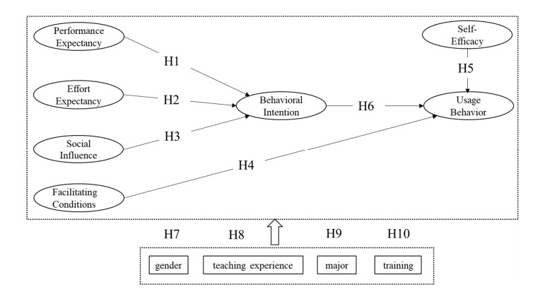
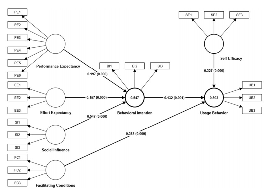
Dynamic mathematics software, such as GeoGebra, is a kind of subject-specific digital tool used for enabling users to create mathematical objects and operate them dynamically and interactively, which is very suitable for mathematics teaching and learning at all school levels, especially at the secondary school level. However, limited research has focused on how multiple influencing factors of secondary school teachers' usage behavior of dynamic mathematics software work together. Based on the unified theory of acceptance and use of technology (UTAUT) model, combined with the concept of self-efficacy, this study proposed a conceptual model used to analyze the factors influencing secondary school teachers' usage behavior of dynamic mathematics software. Valid questionnaire data were provided by 393 secondary school mathematics teachers in the Hunan province of China and analyzed using a partial least squares structural equation modeling (PLS-SEM) method. The results showed that social influence, performance expectancy and effort expectancy significantly and positively affected secondary school teachers' behavioral intentions of dynamic mathematics software, and social influence was the greatest influential factor. In the meantime, facilitating conditions, self-efficacy and behavioral intention had significant and positive effects on secondary school teachers' usage behavior of dynamic mathematics software, and facilitating conditions were the greatest influential factor. Results from the multi-group analysis indicated that gender and teaching experience did not have significant moderating effects on all relationships in the dynamic mathematics software usage conceptual model. However, major had a moderating effect on the relationship between self-efficacy and usage behavior, as well as the relationship between behavioral intention and usage behavior. In addition, training had a moderating effect on the relationship between social influence and behavioral intention. This study has made a significant contribution to the development of a conceptual model that could be used to explore how multiple factors affected secondary school teachers' usage behavior of dynamic mathematics software. It also benefits the government, schools and universities in enhancing teachers' digital teaching competencies.
Citation: Zhiqiang Yuan, Xi Deng, Tianzi Ding, Jing Liu, Qi Tan. Factors influencing secondary school teachers' usage behavior of dynamic mathematics software: A partial least squares structural equation modeling (PLS-SEM) method[J]. Electronic Research Archive, 2023, 31(9): 5649-5684. doi: 10.3934/era.2023287
Dynamic mathematics software, such as GeoGebra, is a kind of subject-specific digital tool used for enabling users to create mathematical objects and operate them dynamically and interactively, which is very suitable for mathematics teaching and learning at all school levels, especially at the secondary school level. However, limited research has focused on how multiple influencing factors of secondary school teachers' usage behavior of dynamic mathematics software work together. Based on the unified theory of acceptance and use of technology (UTAUT) model, combined with the concept of self-efficacy, this study proposed a conceptual model used to analyze the factors influencing secondary school teachers' usage behavior of dynamic mathematics software. Valid questionnaire data were provided by 393 secondary school mathematics teachers in the Hunan province of China and analyzed using a partial least squares structural equation modeling (PLS-SEM) method. The results showed that social influence, performance expectancy and effort expectancy significantly and positively affected secondary school teachers' behavioral intentions of dynamic mathematics software, and social influence was the greatest influential factor. In the meantime, facilitating conditions, self-efficacy and behavioral intention had significant and positive effects on secondary school teachers' usage behavior of dynamic mathematics software, and facilitating conditions were the greatest influential factor. Results from the multi-group analysis indicated that gender and teaching experience did not have significant moderating effects on all relationships in the dynamic mathematics software usage conceptual model. However, major had a moderating effect on the relationship between self-efficacy and usage behavior, as well as the relationship between behavioral intention and usage behavior. In addition, training had a moderating effect on the relationship between social influence and behavioral intention. This study has made a significant contribution to the development of a conceptual model that could be used to explore how multiple factors affected secondary school teachers' usage behavior of dynamic mathematics software. It also benefits the government, schools and universities in enhancing teachers' digital teaching competencies.

| [1] |
S. Timotheou, O. Miliou, Y. Dimitriadis, S. V. Sobrino, N. Giannoutsou, R. Cachia, et al., Impacts of digital technologies on education and factors influencing schools' digital capacity and transformation: A literature review, Educ. Inf. Technol., 28 (2023), 6695–6726. https://doi.org/10.1007/s10639-022-11431-8 doi: 10.1007/s10639-022-11431-8

|
| [2] |
P. Twining, J. Raffaghelli, P. Albion, D. Knezek, Moving education into the digital age: The contribution of teachers' professional development, J. Comput. Assisted Learn., 29 (2013), 426–437. https://doi.org/10.1111/jcal.12031 doi: 10.1111/jcal.12031
|
| [3] |
J. Engelbrecht, S. Llinares, M. C. Borba, Transformation of the mathematics classroom with the internet, ZDM-Math. Educ., 52 (2020), 825–841. https://doi.org/10.1007/s11858-020-01176-4 doi: 10.1007/s11858-020-01176-4
|
| [4] |
M. Beardsley, L. Albo, P. Aragon, D. Hernandez-Leo, Emergency education effects on teacher abilities and motivation to use digital technologies, Br. J. Educ. Technol., 52 (2021), 1455–1477. https://doi.org/10.1111/bjet.13101 doi: 10.1111/bjet.13101
|
| [5] |
S. J. Hegedus, L. Moreno-Armella, The emergence of mathematical structures, Educ. Stud. Math., 77 (2011), 369–388. https://doi.org/10.1007/s10649-010-9297-7 doi: 10.1007/s10649-010-9297-7
|
| [6] | C. Zhou, Children's cognitive abilities in the context of the digital transformation of basic education, Interact. Learn. Environ., 30 (2022), 1–13. |
| [7] | MOE, Standards of Mathematics Curriculum for Compulsory Educaiton (2022 year version)(in Chinese), Beijing Normal University Publishing House, Beijing, China, 2022. |
| [8] | NCTM, Principles and Standards for School Mathematics, NCTM, Reston, VA, 2000. |
| [9] |
O. Birgin, F. Topuz, Effect of the GeoGebra software-supported collaborative learning environment on seventh grade student' geometry achievement, retention and attitudes, J. Educ. Res., 114 (2021), 474–494. https://doi.org/10.1080/00220671.2021.1983505 doi: 10.1080/00220671.2021.1983505
|
| [10] |
O. Birgin, K. U. Yazici, The effect of GeoGebra software-supported mathematics instruction on eighth-grade students' conceptual understanding and retention, J. Comput. Assisted Learn., 37 (2021), 925–939. https://doi.org/10.1111/jcal.12532 doi: 10.1111/jcal.12532
|
| [11] |
R. Bozic, D. Takaci, G. Stankov, Influence of dynamic software environment on students' achievement of learning functions with parameters, Interact. Learn. Environ., 29 (2019), 655–669. https://doi.org/10.1080/10494820.2019.1602842 doi: 10.1080/10494820.2019.1602842
|
| [12] |
E. Cekmez, Investigating the effect of computer-supported instruction on students' understanding of different representations of two-variable inequalities, Interact. Learn. Environ., 31 (2021). https://doi.org/10.1080/10494820.2021.1926288 doi: 10.1080/10494820.2021.1926288
|
| [13] |
M. Demir, Y. Zengin, The effect of a technology-enhanced collaborative learning environment on secondary school students' mathematical reasoning: A mixed method design, Educ. Inf. Technol., 28 (2023), 9855–9883. https://doi.org/10.1007/s10639-023-11587-x doi: 10.1007/s10639-023-11587-x
|
| [14] |
S. Radović, M. Radojičić, K. Veljković, M. Marić, Examining the effects of Geogebra applets on mathematics learning using interactive mathematics textbook, Interact. Learn. Environ., 28 (2020), 32–49. https://doi.org/10.1080/10494820.2018.1512001 doi: 10.1080/10494820.2018.1512001
|
| [15] |
M. S. Uwurukundo, J. F. Maniraho, M. T. Rwibasira, Effect of GeoGebra software on secondary school students' achievement in 3-D geometry, Educ. Inf. Technol., 27 (2022), 5749–5765. https://doi.org/10.1007/s10639-021-10852-1 doi: 10.1007/s10639-021-10852-1
|
| [16] |
H. Zulnaidi, E. Oktavika, R. Hidayat, Effect of use of GeoGebra on achievement of high school mathematics students, Educ. Inf. Technol., 25 (2020), 51–72. https://doi.org/10.1007/s10639-019-09899-y doi: 10.1007/s10639-019-09899-y
|
| [17] |
D. Dalby, M. Swan, Using digital technology to enhance formative assessment in mathematics classrooms, Br. J. Educ. Technol., 50 (2019), 832–845. https://doi.org/10.1111/bjet.12606 doi: 10.1111/bjet.12606
|
| [18] |
D. Juandi, Y. S. Kusumah, M. Tamur, K. S. Perbowo, T. T. Wijaya, A meta-analysis of GeoGebra software decade of assisted mathematics learning: What to learn and where to go?, Heliyon, 7 (2021), e06953. https://doi.org/10.1016/j.heliyon.2021.e06953 doi: 10.1016/j.heliyon.2021.e06953
|
| [19] |
J. S. Pyper, Learning about ourselves: A review of the mathematics teacher in the digital era, Can. J. Sci. Math. Technol. Educ., 17 (2017), 234–242. https://doi.org/10.1080/14926156.2017.1297509 doi: 10.1080/14926156.2017.1297509
|
| [20] |
A. Baccaglini-Frank, To tell a story, you need a protagonist: How dynamic interactive mediators can fulfill this role and foster explorative participation to mathematical discourse, Educ. Stud. Math., 106 (2021), 291–312. https://doi.org/10.1007/s10649-020-10009-w doi: 10.1007/s10649-020-10009-w
|
| [21] |
G. Bozkurt, K. Ruthven, Classroom-based professional expertise: A mathematics teacher's practice with technology, Educ. Stud. Math., 94 (2017), 309–328. https://doi.org/10.1007/s10649-016-9732-5 doi: 10.1007/s10649-016-9732-5
|
| [22] |
I. F. Rahmadi, Z. Lavicza, S. Arkün Kocadere, T. Houghton, M. Hohenwarter, The strengths and weaknesses of user-generated microgames for assisting learning, Educ. Inf. Technol., 27 (2022), 979–995. https://doi.org/10.1007/s10639-021-10635-8 doi: 10.1007/s10639-021-10635-8
|
| [23] |
F. Zhu, B. Xu, The role of dynamic geometry software in teacher-student interactions: Stories from three Chinese mathematics teachers, Sustainability, 15 (2023), 7660. https://doi.org/10.3390/su15097660 doi: 10.3390/su15097660
|
| [24] |
M. J. Bossé, E. S. Young, A. Bayaga, K. Lynch-Davis, A. DeMarte, C. Fountain, Cognitive processes in problem solving in a dynamic mathematics environment, Int. J. Math. Teach. Learn., 21 (2020), 174–196. https://doi.org/10.4256/ijmtl.v21i2.273 doi: 10.4256/ijmtl.v21i2.273
|
| [25] |
M. Cevikbas, G. Kaiser, A systematic review on task design in dynamic and interactive mathematics learning environments (DIMLEs), Mathematics, 9 (2021), 399. https://doi.org/10.3390/math9040399 doi: 10.3390/math9040399
|
| [26] |
D. Martinovic, Z. Karadag, Dynamic and interactive mathematics learning environments: The case of teaching the limit concept, Teach. Math. Its Appl., 31 (2012), 41–48. https://doi.org/10.1093/teamat/hrr029 doi: 10.1093/teamat/hrr029
|
| [27] |
Z. Yuan, J. Liu, X. Deng, T. Ding, T. T. Wijaya, Facilitating conditions as the biggest factor influencing elementary school teachers' usage behavior of dynamic mathematics software in China, Mathematics, 11 (2023), 1536. https://doi.org/10.3390/math11061536 doi: 10.3390/math11061536
|
| [28] |
S. S. Dogruer, D. Akyuz, Mathematical practices of eighth graders about 3D shapes in an argumentation, technology, and design-based classroom environment, Int. J. Sci. Math. Educ., 18 (2020), 1485–1505. https://doi.org/10.1007/s10763-019-10028-x doi: 10.1007/s10763-019-10028-x
|
| [29] |
D. Oner, Tracing the change in discourse in a collaborative dynamic geometry environment: From visual to more mathematical, Int. J. Comput Supported Collab. Learn., 11 (2016), 59–88. https://doi.org/10.1007/s11412-016-9227-5 doi: 10.1007/s11412-016-9227-5
|
| [30] |
A. H. Abdullah, N. S. Misrom, U. H. A. Kohar, M. H. Hamzah, Z. M. Ashari, D. F. Ali, et al., The effects of an inductive reasoning learning strategy assisted by the GeoGebra software on students' motivation for the functional graph Ⅱ topic, IEEE Access, 8 (2020), 143848–143861. https://doi.org/10.1109/ACCESS.2020.3014202 doi: 10.1109/ACCESS.2020.3014202
|
| [31] | P. Shadaan, K. E. Leong, Effectiveness of using GeoGebra on students' understanding in learning circles, Malays. Online J. Educ.Technol., 1 (2013), 1–11. |
| [32] |
E. Cekmez, Using dynamic mathematics software to model a real-world phenomenon in the classroom, Interact. Learn. Environ., 28 (2020), 526–538. https://doi.rog/10.1080/10494820.2019.1674882 doi: 10.1080/10494820.2019.1674882
|
| [33] |
W. Daher, Middle school students' motivation in solving modelling activities with technology, EURASIA J. Math. Sci. Technol. Educ., 17 (2021), em1999. https://doi.org/10.29333/ejmste/11127 doi: 10.29333/ejmste/11127
|
| [34] | M. Hohenwarter, K. J. Fuchs, Combination of dynamic geometry, algebra and calculus in the software system GeoGebra, in Computer Algebra Systems and Dynamic Geometry Systems in Mathematics Teaching, Proceedings of Sprout-Slecting Conference (Sarvari, Cs. Hrsg.), Pecs, Hungary, (2005), 128–133. |
| [35] |
E. Z. Hutkemri, Impact of using GeoGebra on students' conceptual and procedural knowledge of limit function, Mediterr. J. Soc. Sci., 5 (2014), 873–881. https://doi.org/10.5901/mjss.2014.v5n23p873 doi: 10.5901/mjss.2014.v5n23p873
|
| [36] |
E. Çekmez, B.Ö. Bülbül, An example of the use of dynamic mathematics software to create problem-solving environments that serve multiple purposes, Interact. Learn. Environ., 26 (2018), 654–663. https://doi.org/10.1080/10494820.2017.1385029 doi: 10.1080/10494820.2017.1385029
|
| [37] |
H. Jacinto, S. Carreira, Mathematical problem solving with technology: The techno-mathematical fluency of a student-with-GeoGebra, Int. J. Sci. Math. Educ., 15 (2017), 1115–1136. https://doi.org/10.1007/s10763-016-9728-8 doi: 10.1007/s10763-016-9728-8
|
| [38] |
A. Leung, A. M. S. Lee, Students' geometrical perception on a task-based dynamic geometry platform, Educ. Stud. Mathe., 82 (2013), 361–377. https://doi.org/10.1007/s10649-012-9433-7 doi: 10.1007/s10649-012-9433-7
|
| [39] |
J. Olsson, The contribution of reasoning to the utilization of feedback from software when solving mathematical problems, Int. J. Sci. Math. Educ., 16 (2018), 715–735. https://doi.org/10.1007/s10763-016-9795-x doi: 10.1007/s10763-016-9795-x
|
| [40] |
R. Ramirez-Ucles, J. F. Ruiz-Hidalgo, Reasoning, representing, and generalizing in geometric proof problems among 8th grade talented students, Mathematics, 10 (2022), 789. https://doi.org/10.3390/math10050789 doi: 10.3390/math10050789
|
| [41] | Q. Tan, Z. Yuan, A framework on mathematical problem solving with technology and its applications (in Chinese), J. Math. Educ., 30 (2021), 48–54 |
| [42] |
K. K. Chan, S. W. Leung, Dynamic geometry software improves mathematical achievement: Systematic review and meta-analysis, J. Educ. Comput. Res., 51 (2014), 311–325. https://doi.org/10.2190/EC.51.3.c doi: 10.2190/EC.51.3.c
|
| [43] |
A. Sokolowski, Y. Li, V. Willson, The effects of using exploratory computerized environments in grades 1 to 8 mathematics: A meta-analysis of research, Int. J. STEM Educ., 2 (2015), 8. https://doi.org/10.1186/s40594-015-0022-z doi: 10.1186/s40594-015-0022-z
|
| [44] |
A. Dvir, M. Tabach, Learning extrema problems using a non-differential approach in a digital dynamic environment: The case of high-track yet low-achievers, ZDM-Math. Educ., 49 (2017), 785–798. https://doi.org/10.1007/s11858-017-0862-8 doi: 10.1007/s11858-017-0862-8
|
| [45] |
R. S. R. da Silva, L. M. Barbosa, M. C. Borba, A. L. A. Ferreira, The use of digital technology to estimate a value of Pi: Teachers' solutions on squaring the circle in a graduate course in Brazil, ZDM-Math. Educ., 53 (2021), 605–619. https://doi.org/10.1007/s11858-021-01246-1 doi: 10.1007/s11858-021-01246-1
|
| [46] |
M. Turgut, Reinventing geometric linear transformations in a dynamic geometry environment: Multimodal analysis of student reasoning, Int. J. Sci. Math. Educ., 20 (2022), 1203–1223. https://doi.org/10.1007/s10763-021-10185-y doi: 10.1007/s10763-021-10185-y
|
| [47] |
M. Turgut, Sense-making regarding matrix representation of geometric transformations in R2: A semiotic mediation perspective in a dynamic geometry environment, ZDM-Math. Educ., 51 (2019), 1199–1214. https://doi.org/10.1007/s11858-019-01032-0 doi: 10.1007/s11858-019-01032-0
|
| [48] |
Y. Zengin, Construction of proof of the fundamental theorem of calculus using dynamic mathematics software in the calculus classroom, Educ. Inf. Technol., 27 (2022), 2331–2366. https://doi.org/10.1007/s10639-021-10666-1 doi: 10.1007/s10639-021-10666-1
|
| [49] |
O. Birgin, H. Acar, The effect of computer-supported collaborative learning using GeoGebra software on 11th grade students' mathematics achievement in exponential and logarithmic functions, Int. J. Math. Educ. Sci. Technol., 53 (2022), 872–889. https://doi.org/10.1080/0020739X.2020.1788186 doi: 10.1080/0020739X.2020.1788186
|
| [50] |
M. Mthethwa, A. Bayaga, M. J. Bossé, D. Williams, GeoGebra for learning and teaching: A parallel investigation, South African J. Educ., 40 (2020), 1669. https://doi.org/10.15700/saje.v40n2a1669 doi: 10.15700/saje.v40n2a1669
|
| [51] |
K. Acikgul, R. Aslaner, Effects of Geogebra supported micro teaching applications and technological pedagogical content knowledge (TPACK) game practices on the TPACK levels of prospective teachers, Educ. Inf. Technol., 25 (2020), 2023–2047. https://doi.org/10.1007/s10639-019-10044-y doi: 10.1007/s10639-019-10044-y
|
| [52] |
O. Erkek, M. I. Bostan, Prospective middle school mathematics teachers' global argumentation structures, Int. J. Sci. Math. Educ., 17 (2019), 613–633. https://doi.org/10.1007/s10763-018-9884-0 doi: 10.1007/s10763-018-9884-0
|
| [53] |
S. B. Khoza, A. T. Biyela, Decolonising technological pedagogical content knowledge of first year mathematics students, Educ. Inf. Technol., 25 (2020), 2665–2679. https://doi.org/10.1007/s10639-019-10084-4 doi: 10.1007/s10639-019-10084-4
|
| [54] |
N. C. Verhoef, F. Coenders, J. M. Pieters, D. van Smaalen, D. O. Tall, Professional development through lesson study: Teaching the derivative using GeoGebra, Prof. Develop. Educ., 41 (2015), 109–126. https://doi.org/10.1080/19415257.2014.886285 doi: 10.1080/19415257.2014.886285
|
| [55] |
Y. Zengin, Development of mathematical connection skills in a dynamic learning environment, Educ. Inf. Technol., 24 (2019), 2175–2194. http://doi.org/10.1007/s10639-019-09870-x doi: 10.1007/s10639-019-09870-x
|
| [56] |
Y. Zengin, Effectiveness of a professional development course based on information and communication technologies on mathematics teachers' skills in designing technology-enhanced task, Educ. Inf. Technol., 28 (2023). https://doi.org/10.1007/s10639-023-11728-2 doi: 10.1007/s10639-023-11728-2
|
| [57] |
S. Gokce, P. Guner, Dynamics of GeoGebra ecosystem in mathematics education, Educ. Inf. Technol., 27 (2022), 5301–5323. https://doi.org/10.1007/s10639-021-10836-1 doi: 10.1007/s10639-021-10836-1
|
| [58] |
A. Yohannes, H. L. Chen, GeoGebra in mathematics education: A systematic review of journal articles published from 2010 to 2020, Interact. Learn. Environ., 29 (2021), 1–16. https://doi.org/10.1080/10494820.2021.2016861 doi: 10.1080/10494820.2021.2016861
|
| [59] |
M. D. Gurer, Examining technology acceptance of pre-service mathematics teachers in Turkey: A structural equation modeling approach, Educ. Inf. Technol., 26 (2021), 4709–4729. https://doi.org/10.1007/s10639-021-10493-4 doi: 10.1007/s10639-021-10493-4
|
| [60] |
K. F. Hollebrands, The role of a dynamic software program for geometry in the strategies high school mathematics students employ, J. Res. Math. Educ., 38 (2007), 164–192. https://doi.org/10.2307/30034955 doi: 10.2307/30034955
|
| [61] |
F. Ulusoy, İ. B. Turuş, The mathematical and technological nature of tasks containing the use of dynamic geometry software in middle and secondary school mathematics textbooks, Educ. Inf. Technol., 27 (2022), 11089–11113. https://doi.org/10.1007/s10639-022-11070-z doi: 10.1007/s10639-022-11070-z
|
| [62] |
K. Ruthven, R. Deaney, S. Hennessy, Using graphing software to teach about algebraic forms: A study of technology-supported practice in secondary-school mathematics, Educ. Stud. Math., 71 (2009), 279–297. https://doi.org/10.1007/s10649-008-9176-7 doi: 10.1007/s10649-008-9176-7
|
| [63] |
J. Hohenwarter, M. Hohenwarter, Z. Lavicza, Introducing dynamic mathematics software to second school teachers: The case of GeoGebra, J. Comput. Math. Sci. Teach., 28 (2008), 135–146. https://doi.org/10.13140/RG.2.2.15003.05921 doi: 10.13140/RG.2.2.15003.05921
|
| [64] |
R. Pierce, K. Stacey, Mapping pedagogical opportunities provided by mathematics analysis software, Int. J. Comput. Math. Learn., 15 (2010), 1–20. https://doi.org/10.1007/s10758-010-9158-6 doi: 10.1007/s10758-010-9158-6
|
| [65] |
R. Marrades, Á. Gutiérrez, Proofs produced by secondary school students learning geometry in a dynamic computer environment, Educ. Stud. Math., 44 (2000), 87–125. https://doi.org/10.1023/A:1012785106627 doi: 10.1023/A:1012785106627
|
| [66] |
G. G. Nagar, S. Hegedus, C. H. Orrill, High school mathematics teachers' discernment of invariant properties in a dynamic geometry environment, Educ. Stud. Math., 111 (2022), 127–145. https://doi.org/10.1007/s10649-022-10144-6 doi: 10.1007/s10649-022-10144-6
|
| [67] |
M. S. Alabdulaziz, S. M. Aldossary, S. A. Alyahya, H. M. Althubiti, The effectiveness of the GeoGebra programme in the development of academic achievement and survival of the learning impact of the mathematics among secondary stage students, Educ. Inf. Technol., 26 (2021), 2685–2713. https://doi.org/10.1007/s10639-020-10371-5 doi: 10.1007/s10639-020-10371-5
|
| [68] |
F. D. Davis, Perceived usefulness, perceived ease of use, and user acceptance of information technology, MIS Quarterly, 13 (1989), 319–340. https://doi.org/10.2307/249008 doi: 10.2307/249008
|
| [69] |
F. D. Davis, R. P. Bagozzi, P. R. Warshaw, User acceptance of computer technology: A comparison of two theoretical models, Manage. Sci., 35 (1989), 982–1003. https://doi.org/10.1287/mnsc.35.8.982 doi: 10.1287/mnsc.35.8.982
|
| [70] |
V. Venkatesh, F. D. Davis, A theoretical extension of the technology acceptance model: Four longitudinal field studies, Manage. Sci., 46 (2000), 186–204. https://doi.org/10.1287/mnsc.46.2.186.11926 doi: 10.1287/mnsc.46.2.186.11926
|
| [71] |
I. Ajzen, The theory of planned behavior, Organ. Behav. Hum. Dec. Processes, 50 (1991), 179–211. https://doi.org/10.1016/0749-5978(91)90020-T doi: 10.1016/0749-5978(91)90020-T
|
| [72] | E. M. Rogers, Diffusion of Innovations, The Free Press, New York, 1963. |
| [73] |
V. Venkatesh, M.G. Morris, G. B. Davis, F. D. Davis, User acceptance of information technology: Toward a unified view, MIS Quarterly, 27 (2003), 425–478. https://doi.org/10.5555/2017197.2017202 doi: 10.5555/2017197.2017202
|
| [74] |
V. Venkatesh, J. Y. L. Thong, X. Xu, Consumer acceptance and use of information technology: Extending the unified theory of acceptance and use of technology, MIS Quarterly, 36 (2012), 157–178. https://doi.org/10.2307/41410412 doi: 10.2307/41410412
|
| [75] |
A. M. Al-Rahmi, A. Shamsuddin, E. Wahab, W. M. Al-Rahmi, U. Alturki, A. Aldraiweesh, et al., Integrating the role of UTAUT and TTF model to evaluate social media use for teaching and learning in higher education, Front. Public Health, 10 (2022), 905968. https://doi.org/10.3389/fpubh.2022.905968 doi: 10.3389/fpubh.2022.905968
|
| [76] |
L. Wan, S. Xie, A. Shu, Toward an understanding of university students' continued Intention to use MOOCs: When UTAUT model meets TTF model, SAGE Open, 10 (2020). https://doi.org/10.1177/2158244020941858 doi: 10.1177/2158244020941858
|
| [77] |
M. D. Williams, N. P. Rana, Y. K. Dwivedi, The unified theory of acceptance and use of technology (UTAUT): A literature review, J. Enterp. Inf. Manage., 28 (2015), 443–488. https://doi.org/10.1108/JEIM-09-2014-0088 doi: 10.1108/JEIM-09-2014-0088
|
| [78] |
C. M. Chao, Factors determining the behavioral intention to use mobile learning: An application and extension of the UTAUT model, Front. Psychol., 10 (2019), 1652. https://doi.org/10.3389/fpsyg.2019.01652 doi: 10.3389/fpsyg.2019.01652
|
| [79] |
A. Kundu, T. Bej, K. N. Dey, Investigating effects of self-efficacy and infrastructure on teachers' ICT use: An extension of UTAUT, Int. J. Web-Based Learn. Teach. Technol. (IJWLTT), 16 (2021), 21. https://doi.org/10.4018/IJWLTT.20211101.oa10 doi: 10.4018/IJWLTT.20211101.oa10
|
| [80] |
A. Clark-Wilson, O. Robutti, M. Thomas, Teaching with digital technology, ZDM-Math. Educ., 52 (2020), 1223–1242. https://doi.org/10.1007/s11858-020-01196-0 doi: 10.1007/s11858-020-01196-0
|
| [81] |
T. T. Wijaya, Y. Zhou, T. Houghton, R. Weinhandl, Z. Lavicza, F.D. Yusop, Factors affecting the use of digital mathematics textbooks in Indonesia, Mathematics, 10 (2022), 1808. https://doi.org/10.3390/math10111808 doi: 10.3390/math10111808
|
| [82] |
Ş. B. Tosuntaş, E. Karadağ, S. Orhan, The factors affecting acceptance and use of interactive whiteboard within the scope of FATIH project: A structural equation model based on the unified theory of acceptance and use of technology, Comput. Educ., 81 (2015), 169–178. https://doi.org/10.1016/j.compedu.2014.10.009 doi: 10.1016/j.compedu.2014.10.009
|
| [83] |
V. Venkatesh, H. Bala, Technology acceptance model 3 and a research agenda on interventions, Decis. Sci., 39 (2008), 273–315. https://doi.org/10.1111/j.1540-5915.2008.00192.x doi: 10.1111/j.1540-5915.2008.00192.x
|
| [84] |
M. A. O. Abbad, Using the UTAUT model to understand students' usage of e-learning systems in developing countries, Educ. Inf. Technol., 26 (2021), 7205–7224. https://doi.org/10.1007/s10639-021-10573-5 doi: 10.1007/s10639-021-10573-5
|
| [85] |
T. T. Wijaya, R. Weinhandl, Factors influencing students's continuous intentions for using micro-lectures in the post-COVID-19 period: A modification of the UTAUT-2 approach, Electronics, 11 (2022), 1924. https://doi.org/10.3390/electronics11131924 doi: 10.3390/electronics11131924
|
| [86] |
T. T. Wijaya, Y. Cao, R. Weinhandl, E. Yusron, Z. Lavicza, Applying the UTAUT model to understand factors affecting micro-lecture usage by mathematics teachers in China, Mathematics, 10 (2022), 1008. https://doi.org/10.3390/math10071008 doi: 10.3390/math10071008
|
| [87] |
T. Zhou, Y. Lu, B. Wang, Integrating TTF and UTAUT to explain mobile banking user adoption, Comput. Hum. Behav., 26 (2010), 760–767. https://doi.org/10.1016/j.chb.2010.01.013 doi: 10.1016/j.chb.2010.01.013
|
| [88] |
H. J. Lai, Investigating older adults' decisions to use mobile devices for learning, based on the unified theory of acceptance and use of technology, Int. Learn. Environ., 28 (2020), 890–901. https://doi.org/10.1080/10494820.2018.1546748 doi: 10.1080/10494820.2018.1546748
|
| [89] |
B. Šumak, A. Šorgo, The acceptance and use of interactive whiteboards among teachers: Differences in UTAUT determinants between pre- and post-adopters, Comput. Hum. Behav., 64 (2016), 602–620. https://doi.org/10.1016/j.chb.2016.07.037 doi: 10.1016/j.chb.2016.07.037
|
| [90] |
A. Gunasinghe, J. A. Hamid, A. Khatibi, S. M. F. Azam, The viability of UTAUT-3 in understanding the lecturer's acceptance and use of virtual learning environments, Int. J. Technol. Enhanced Learn., 12 (2020), 458–481. https://doi.org/10.1504/IJTEL.2020.110056 doi: 10.1504/IJTEL.2020.110056
|
| [91] |
J. Kim, K. S. S. Lee, Conceptual model to predict Filipino teachers' adoption of ICT-based instruction in class: Using the UTAUT model, Asia Pac. J. Educ., 42 (2022), 699–713. https://doi.org/10.1080/02188791.2020.1776213 doi: 10.1080/02188791.2020.1776213
|
| [92] |
A. Bandura, The explanatory and predictive scope of self-efficacy theory, J. Soc. Clin. Psychol., 4 (1986), 359–373. https://doi.org/10.1521/jscp.1986.4.3.359 doi: 10.1521/jscp.1986.4.3.359
|
| [93] |
J. Wu, H. Du, Toward a better understanding of behavioral intention and system usage constructs, Eur. J. Inf. Syst., 21 (2012), 680–698. https://doi.org/10.1057/ejis.2012.15 doi: 10.1057/ejis.2012.15
|
| [94] |
W. H. Loo, P. H. P. Yeow, S. C. Chong, User acceptance of Malaysian government multipurpose smartcard applications, Gov. Inf. Q., 26 (2009), 358–367. https://doi.org/10.1016/j.giq.2008.07.004 doi: 10.1016/j.giq.2008.07.004
|
| [95] |
S. Lakhal, H. Khechine, J. Mukamurera, Explaining persistence in online courses in higher education: A difference-in-differences analysis, Int. J. Educ. Technol. Higher Educ., 18 (2021), 19. https://doi.org/10.1186/s41239-021-00251-4 doi: 10.1186/s41239-021-00251-4
|
| [96] |
V. Marinković, A. Đorđević, Z. Kalinić, The moderating effects of gender on customer satisfaction and continuance intention in mobile commerce: A UTAUT-based perspective, Technol. Anal. Strategic Manage., 32 (2020), 306–318. https://doi.org/10.1080/09537325.2019.1655537 doi: 10.1080/09537325.2019.1655537
|
| [97] |
S. J. Jang, M. F. Tsai, Reasons for using or not using interactive whiteboards: Perspectives of Taiwanese elementary mathematics and science teachers, Australas. J. Educ. Technol., 28 (2012), 1451–1465. https://doi.org/10.14742/ajet.781 doi: 10.14742/ajet.781
|
| [98] |
S. Hu, K. Laxman, K. Lee, Exploring factors affecting academics' adoption of emerging mobile technologies: An extended UTAUT perspective, Educ. Inf. Technol., 25 (2020), 4615–4635. https://doi.org/10.1007/s10639-020-10171-x doi: 10.1007/s10639-020-10171-x
|
| [99] | Z. Yuan, S. Li, Developing prospective mathematics teachers' technological pedagogical content knowledge (TPACK): A case of normal distribution, in The 12th International Congress on Mathematical Education, (2012), 5804–5813. |
| [100] |
C. Y. Lee, M. J. Chen, Developing a questionnaire on technology-integrated mathematics instruction: A case study of the AMA training course in Xinjiang and Taiwan, Br. J. Educ. Technol., 46 (2016), 1287–1303. https://doi.org/10.1111/bjet.12339 doi: 10.1111/bjet.12339
|
| [101] |
K. Sungur Gül, H. Ateş, An examination of the effect of technology-based STEM education training in the framework of technology acceptance model, Educ. Inf. Technol., 28 (2023), 8761–8787. https://doi.org/10.1007/s10639-022-11539-x doi: 10.1007/s10639-022-11539-x
|
| [102] | W. W. Chin, The partial least squares approach to structural equation modeling, in Mordern Methods for Business Research, Erlbaum, (1998), 295–358. |
| [103] |
J. F. Hair, C. M. Ringle, M. Starstedt, PLS-SEM: Indeed a silver bullet, J. Mark. Theory Practice, 19 (2011), 139–151. https://doi.org/10.2753/MTP1069-6679190202 doi: 10.2753/MTP1069-6679190202
|
| [104] |
J. F. Hair, M. Sarstedt, C. M. Ringle, J. A. Mena, An assessment of the use of partial least squares structural equation modeling in marketing research, J. Acad. Mark Sci., 40 (2012), 414–433. https://doi.org/10.1007/s11747-011-0261-6 doi: 10.1007/s11747-011-0261-6
|
| [105] |
J. F. Hair, J. J. Risher, M. Sarstedt, C. M. Ringle, When to use and how to report the results of PLS-SEM, Eur. Business Rev., 31 (2019), 2–24. https://doi.org/10.1108/EBR-11-2018-0203 doi: 10.1108/EBR-11-2018-0203
|
| [106] | J. F. Hair, G. T. M. Hult, C.M. Ringle, M. Sarstedt, A Primer on Partial Least Squares Structural Equation Modeling (PLS-SEM), 3rd edition, Sage Publications, Thousand oaks, CA, 2022. |
| [107] | J. F. Hair, M. Sarstedt, C. M. Ringle, S. P. Gudergan, Advanced Issues in Partial Least Squares Structural Equation Modeling, 2nd edition, SAGE, Thousand Oaks, CA, 2023. |
| [108] |
H. M. Lin, M. H. Lee, J. C. Liang, H. Y. Chang, P. Huang, C. C. Tsai, A review of using partial least square structural equation modeling in e-learning research, Br. J. Educ. Technol., 51 (2020), 1354–1372. https://doi.org/10.1111/bjet.12890 doi: 10.1111/bjet.12890
|
| [109] | H. Wold, Partial least squares, in Encyclopedia of Statistical Sciences, (Eds. S. Kotz and N. L. Johnson), Wiley, (1985), 581–591. |
| [110] | Z. Karadag, D. McDougall, GeoGebra as a cognitive tool: Where cognitive theories and technology meet, in Model-Centered Learning: Pathways to Mathematical Understanding Using GeoGebra, (Eds. L. Bu and R. Schoen), Sense Publishers, (2011), 169–181. |
| [111] |
Z. A. Reis, S. Ozdemir, Using GeoGebra as an information technology tool: Parabola teaching, Proc. Soc. Behav. Sci., 9 (2010), 565–572. https://doi.org/10.1016/j.sbspro.2010.12.198 doi: 10.1016/j.sbspro.2010.12.198
|
| [112] |
R. Ziatdinov, J. R. Valles, Synthesis of modeling, visualization, and programming in GeoGebra as an effective approach for teaching and learning STEM topics, Mathematics, 10 (2022), 398. https://doi.org/10.3390/math10030398 doi: 10.3390/math10030398
|
| [113] |
M. Pittalis, Extending the technology acceptance model to evaluate teachers' intention to use dynamic geometry software in geometry teaching, Int. J. Math. Educ. Sci. Technol., 52 (2021), 1385–1404. https://doi.org/10.1080/0020739X.2020.1766139 doi: 10.1080/0020739X.2020.1766139
|
| [114] | Z. Yuan, M. Milner-Bolotin, A study of a TPACK-based subject-specific educational technology course and its implications: The case of "teaching mathematics and science through technology" course at the University of British Columbia (in Chinese), J. Math. Educ., 29 (2020), 23–28 |
| [115] |
Z. Drezner, O. Turel, D. Zerom, A modified Kolmogorov–Smirnov test for normality, Commun. Stat. Simul. Comput., 39 (2010), 693–704. https://doi.org/10.1080/03610911003615816 doi: 10.1080/03610911003615816
|
| [116] | B. M. Byrne, Structural Equation Modeling With AMOS: Basic Concepts, Applications, and Programming, 3rd edition, Routledge, New York, 2016. |
| [117] |
M. A. Moteri, M. Alojail, Factors influencing the supply chain management in e-health using UTAUT model, Electron. Res. Arch., 31 (2023), 2855–2877. https://doi.org/10.3934/era.2023144 doi: 10.3934/era.2023144
|
| [118] |
J. M. Santos-Jaén, A. León-Gómez, D. Ruiz-Palomo, F. García-Lopera, M. D. V. Martínez, Exploring information and communication technologies as driving forces in hotel SMEs performance: Influence of corporate social responsibility, Mathematics, 10 (2022), 3629. https://doi.org/10.3390/math10193629 doi: 10.3390/math10193629
|
| [119] |
M. D. Valls Martínez, P. A. Martín-Cervantes, A. M. Sánchez Pérez, M. D. Martínez Victoria, Learning mathematics of financial operations during the COVID-19 era: An assessment with partial least squares structural equation modeling, Mathematics, 9 (2021), 2120. https://doi.org/10.3390/math9172120 doi: 10.3390/math9172120
|
| [120] |
T. T. Wijaya, B. Yu, F. Xu, Z. Yuan, M. Mailizar, Analysis of factors affecting academic performance of mathematics education doctoral students: A structural equation modeling approach, Int. J. Environ. Res. Pub. Health, 20 (2023), 4518. https://doi.org/10.3390/ijerph20054518 doi: 10.3390/ijerph20054518
|
| [121] |
L. J. Cronbach, Coefficient alpha and the internal structure of tests, Psychometrika, 16 (1951), 297–334. https://doi.org/10.1007/BF02310555 doi: 10.1007/BF02310555
|
| [122] |
T. K. Dijkstra, J. Henseler, Consistent partial least squares path modeling, MIS Q., 39 (2015), 297–316. https://doi.org/10.25300/MISQ/2015/39.2.02 doi: 10.25300/MISQ/2015/39.2.02
|
| [123] |
C. E. Werts, R. L. Linn, K. G. Jöreskog, Intraclass reliability estimates: Testing structural assumptions, Educ. Psychol. Meas., 34 (1974), 25–33. https://doi.org/10.1177/001316447403400104 doi: 10.1177/001316447403400104
|
| [124] |
C. Fornell, D. F. Larcker, Evaluating structural equation models with unobservable variables and measurement error, J. Mark. Res., 18 (1981), 39–50. https://doi.org/10.1177/002224378101800104 doi: 10.1177/002224378101800104
|
| [125] |
J. Henseler, C. M. Ringle, M. Sarstedt, A new criterion for assessing discriminant validity in variance-based structural equation modeling, J. Acad. Mark. Sci., 43 (2015), 115–135. https://doi.org/10.1007/s11747-014-0403-8 doi: 10.1007/s11747-014-0403-8
|
| [126] |
J. Henseler, G. Hubona, P. A. Ray, Using PLS path modeling in new technology research: Updated guidelines, Ind. Manage. Data Syst., 116 (2016), 2–20. https://doi.org/10.1108/IMDS-09-2015-0382 doi: 10.1108/IMDS-09-2015-0382
|
| [127] | P. M. Bentler, EQS Structural Equations Program Manual, CA: Multivariate Software, Encino, CA, 1995. |
| [128] |
P. M. Bentler, D. G. Bonett, Significance tests and goodness of fit in the analysis of covariance structures, Psychol. Bull., 88 (1980), 588–606. https://doi.org/10.1037/0033-2909.88.3.588 doi: 10.1037/0033-2909.88.3.588
|
| [129] |
F. Schuberth, M. E. Rademaker, J. Henseler, Assessing the overall fit of composite models estimated by partial least squares path modeling, Eur. J. Mark., 57 (2023), 1678–1702. https://doi.org/10.1108/EJM-08-2020-0586 doi: 10.1108/EJM-08-2020-0586
|
| [130] |
G. Shmueli, M. Sarstedt, J. F. Hair, J. H. Cheah, H. Ting, S. Vaithilingam, et al., Predictive model assessment in PLS-SEM: Guidelines for using PLSpredict, Eur. J. Mark., 53 (2019), 2322-2347. https://doi.org/10.1108/EJM-02-2019-0189 doi: 10.1108/EJM-02-2019-0189
|
| [131] | J. Henseler, C. M. Ringle, R. R. Sinkovics, The use of partial least squares path modeling in international marketing, in New Challenges to International Marketing, (Eds. R. R. Sinkovics and P. N. Ghauri), Emerald Group Publishing Limited, Bingley, (2009), 277–319. |
| [132] | W. W. Chin, J. Dibbern, A permutation-based procedure for multi-group PLS analysis: Results of tests of differences on simulated data and a cross cultural analysis of the sourcing of information system services between Germany and the USA, (Eds. V. Esposito Vinzi, et al.), Springer, Berlin, (2010). |
| [133] | M. Sarstedt, J. Henseler, C. M. Ringle, Multigroup analysis in partial least squares (PLS) path modeling: Alternative methods and empirical results, in Measurement and Research Methods in International Marketing, (Eds. M. Sarstedt, M. Schwaiger and C. R. Taylor), Emerald Group Publishing Limited, (2011), 195–218. |
| [134] |
J. M. Bland, D. G. Altman, Multiple significance tests: The Bonferroni method, BMJ, 310 (1995), 170. https://doi.org/10.1136/bmj.310.6973.170 doi: 10.1136/bmj.310.6973.170
|
| [135] | J. F. Hair, W. Black, B. Babin, R. Anderson, Multivariate Data Analysis, 8th edition, Cengage Learning EMEA, Hampshire, United Kingdom, 2019. |
Figures(2) / Tables(17)
Zhiqiang Yuan, Xi Deng, Tianzi Ding, Jing Liu, Qi Tan. Factors influencing secondary school teachers' usage behavior of dynamic mathematics software: A partial least squares structural equation modeling (PLS-SEM) method[J]. Electronic Research Archive, 2023, 31(9): 5649-5684. doi: 10.3934/era.2023287


 DownLoad: