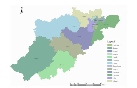
The scale of tourism has continued to expand in recent years, and many associated activities cause damage to the natural environment. The tourism, economy and natural environment constitute a system: destruction of the natural environment reduces the value of tourism and a lack of tourism affects the development of the economy. To explore the relationship between the tourism, economy and natural environment, and to explore possibilities for sustainable development, this paper takes Hangzhou, a tourist city in China, as a research object. An analysis of time series data is carried out. First, the tourism, economy and natural environment subsystems are constructed by extracting time series data acquired between 2010 and 2020. Second, a tourism evaluation model with coupled economic and natural environment data is constructed and the coupling degree and coupling coordination level in Hangzhou are evaluated. Third, the time series of each subsystem and the coupling coordination level of the whole system are analyzed. Finally, an optimization strategy is proposed for the coupled coordinated development of the tourism, economy and natural environment in Hangzhou. A key result is that the tertiary industry represented by tourism has become the main source of local income. Hangzhou's tourism coupling coordination level has changed from slight disorder in 2010 to good in 2020. It is also found that the COVID-19 pandemic has become a major factor restricting the development of tourism. Before the outbreak of COVID-19, Hangzhou's tourism industry and economy were synchronized. After the outbreak of COVID-19, both the number of tourists and tourism revenue in Hangzhou fell by nearly 15%.
Citation: Haifeng Song, Weijia Wang, Jiaqi Zhu, Cong Ren, Xin Li, Wenyi Lou, Weiwei Yang, Lei Du. Research on the sustainable development of tourism coupled with economic and environment data——a case study of Hangzhou[J]. Mathematical Biosciences and Engineering, 2023, 20(12): 20852-20880. doi: 10.3934/mbe.2023923
The scale of tourism has continued to expand in recent years, and many associated activities cause damage to the natural environment. The tourism, economy and natural environment constitute a system: destruction of the natural environment reduces the value of tourism and a lack of tourism affects the development of the economy. To explore the relationship between the tourism, economy and natural environment, and to explore possibilities for sustainable development, this paper takes Hangzhou, a tourist city in China, as a research object. An analysis of time series data is carried out. First, the tourism, economy and natural environment subsystems are constructed by extracting time series data acquired between 2010 and 2020. Second, a tourism evaluation model with coupled economic and natural environment data is constructed and the coupling degree and coupling coordination level in Hangzhou are evaluated. Third, the time series of each subsystem and the coupling coordination level of the whole system are analyzed. Finally, an optimization strategy is proposed for the coupled coordinated development of the tourism, economy and natural environment in Hangzhou. A key result is that the tertiary industry represented by tourism has become the main source of local income. Hangzhou's tourism coupling coordination level has changed from slight disorder in 2010 to good in 2020. It is also found that the COVID-19 pandemic has become a major factor restricting the development of tourism. Before the outbreak of COVID-19, Hangzhou's tourism industry and economy were synchronized. After the outbreak of COVID-19, both the number of tourists and tourism revenue in Hangzhou fell by nearly 15%.

| [1] |
J. M. Ahmed, A review and situational analysis of Thomas cook business failure, a successful business model for 178 years: A case study, Int. J. Inc. Dev., 6 (2020), 60–38. https://doi.org/10.30954/2454-4132.1.2020.9 doi: 10.30954/2454-4132.1.2020.9

|
| [2] |
F. Higgins-Desbiolles, The "war over tourism": challenges to sustainable tourism in the tourism academy after COVID-19, J. Sustain. Tour., 29 (2020), 551–569. https://doi.org/10.1080/09669582.2020.1803334 doi: 10.1080/09669582.2020.1803334
|
| [3] |
K. Aliyev, N. Ahmadova, Testing tourism-led economic growth and economic-driven tourism growth hypotheses: The case of Georgia, Tourism, 68 (2020), 43–57. https://doi.org/10.37741/t.68.1.4 doi: 10.37741/t.68.1.4
|
| [4] | Q. Dang, C. Wu, A research on the Tourists' perceived evaluation and management of safety risks for Tourism cities: A case study of HangZhou, in 2nd International Forum on Management, Education and Information Technology Application (IFMEITA 2017), (2018), 55–65. https://doi.org/10.2991/ifmeita-17.2018.10 |
| [5] |
Z. W. Wang, Interaction between the tourism industry and ecological environment based on the Complicated Adaptation System (CAS) theory: A case study on Henan Province, China, Nat. Environ. Pollut. Technol., 19 (2020), 1039–1045. https://doi.org/10.46488/NEPT.2020.v19i03.014 doi: 10.46488/NEPT.2020.v19i03.014
|
| [6] |
D. Wang, X. Zhao, Affective video recommender systems: A survey, Front. Neurosci., 16 (2022), 1–20. https://doi.org/10.3389/fnins.2022.984404 doi: 10.3389/fnins.2022.984404
|
| [7] |
Y. F. Shen, Measurement of tourism industry-ecological environment coupling degree and management and control measures for tourism environment: A case study of Henan Province, China, Nat. Environ. Pollut. Technol., 19 (2020), 857–864. https://doi.org/10.46488/NEPT.2020.V19I02.045 doi: 10.46488/NEPT.2020.V19I02.045
|
| [8] |
Q. Cheng, Z. Luo, L. Xiang, Spatiotemporal differentiation of coupling and coordination relationship of the tea industry–Tourism–ecological environment system in Fujian Province, China, Sustainability (Switzerland), 13 (2021), 10628. https://doi.org/10.3390/su131910628 doi: 10.3390/su131910628
|
| [9] | X. Yang, Study on the coordinated development of regional economic, tourism and ecology coupling: Taking Henan Province as an example, Fresen. Environ. Bull., 39 (2021), 210–215. |
| [10] |
L. Sun, L. Zeng, H. Zhou, L. Zhang, Strip thickness prediction method based on improved border collie optimizing LSTM, PeerJ Comput. Sci., 2022 (2022), 1–22. https://doi.org/10.7717/peerj-cs.1114 doi: 10.7717/peerj-cs.1114
|
| [11] |
X. Qin, X. M. Li, Evaluate on the decoupling of tourism economic development and ecological-environmental stress in China, Sustainability (Switzerland), 13 (2021), 2149. https://doi.org/10.3390/su13042149 doi: 10.3390/su13042149
|
| [12] |
H. Song, W. Yang, GSCCTL: a general semi-supervised scene classification method for remote sensing images based on clustering and transfer learning, Int. J. Remote Sens., 43 (2022), 15-16. https://doi.org/10.1080/01431161.2021.2019851 doi: 10.1080/01431161.2021.2019851
|
| [13] |
P. del Vecchio, C. Malandugno, G. Passiante, G. Sakka, Circular economy business model for smart tourism: the case of Ecobnb, EuroMed J. Bus., 17 (2022), 88–104. https://doi.org/10.1108/EMJB-09-2020-0098 doi: 10.1108/EMJB-09-2020-0098
|
| [14] |
J. M. Beall, B. B. Boley, A. C. Landon, K. M. Woosnam, What drives ecotourism: environmental values or symbolic conspicuous consumption?, J. Sustain. Tour., 29 (2021), 1215–1234. https://doi.org/10.1080/09669582.2020.1825458 doi: 10.1080/09669582.2020.1825458
|
| [15] |
V. Lopes, S. M. Pires, R. Costa, A strategy for a sustainable tourism development of the Greek Island of Chios, Tourism, 68 (2020), 243–260. https://doi.org/10.37741/T.68.3.1 doi: 10.37741/T.68.3.1
|
| [16] |
B. K. Mudzengi, E. Gandiwa, N. Muboko, C. N. Mutanga, Towards sustainable community conservation in tropical savanna ecosystems: a management framework for ecotourism ventures in a changing environment, Environ., Dev. Sustain., 23 (2021), 3028–3047. https://doi.org/10.1007/s10668-020-00772-4 doi: 10.1007/s10668-020-00772-4
|
| [17] |
S. K. Mallick, S. Rudra, R. Samanta, Sustainable ecotourism development using SWOT and QSPM approach: A study on Rameswaram, Tamil Nadu, Int. J. Geo. Park., 8 (2020), 185–193. https://doi.org/10.1016/j.ijgeop.2020.06.001 doi: 10.1016/j.ijgeop.2020.06.001
|
| [18] | J. Yushi, Z. Yuzong, Centennial research process of tourism geography in Japan, Geogr. Res., 37 (2018), 2039–2057. |
| [19] |
S. Shigeru, Kureha, M.: Development process of Ski resorts: A comparative study of Japan and Austria, Geogr. Rev. Japan Series A, 90 (2017), 519–523. https://doi.org/10.4157/grj.90.519 doi: 10.4157/grj.90.519
|
| [20] |
J. Zhang, Y. Zhang, Assessing the low-carbon tourism in the tourism-based urban destinations, J. Clean. Prod., 276 (2020), 124303. https://doi.org/10.1016/j.jclepro.2020.124303 doi: 10.1016/j.jclepro.2020.124303
|
| [21] |
K. Bhaktikul, S. Aroonsrimorakot, M. Laiphrakpam, W. Paisantanakij, Toward a low-carbon tourism for sustainable development: a study based on a royal project for highland community development in Chiang Rai, Thailand, Environ., Dev. Sustain., 23 (2021), 743–762. https://doi.org/10.1007/s10668-020-01083-4 doi: 10.1007/s10668-020-01083-4
|
| [22] |
H. Sun, T. Chen, C. N. Wang, Spatial impact of digital finance on carbon productivity, Geosci. Front., (2023), 101674. https://doi.org/https://doi.org/10.1016/j.gsf.2023.101674 doi: 10.1016/j.gsf.2023.101674
|
| [23] | V. M. Quintana, Eco-cultural tourism: Sustainable development and promotion of natural and cultural heritage, in Tourism, IntechOpen, (2020), 1–17. https://doi.org/10.5772/intechopen.93897 |
| [24] |
K. J. Wu, Y. Zhu, Q. Chen, M. L. Tseng, Building sustainable tourism hierarchical framework: Coordinated triple bottom line approach in linguistic preferences, J. Clean. Prod., 229 (2019), 157–168. https://doi.org/10.1016/j.jclepro.2019.04.212 doi: 10.1016/j.jclepro.2019.04.212
|
| [25] |
A. Csikósová, M. Janošková, K. Čulková, Providing of tourism organizations sustainability through triple bottom line approach, Entrep. Sustain. Iss., 8 (2020), 764–776. https://doi.org/10.9770/jesi.2020.8.2(46) doi: 10.9770/jesi.2020.8.2(46)
|
| [26] |
B. Grah, V. Dimovski, J. Peterlin, Managing Sustainable Urban Tourism Development: The Case of Ljubljana, Sustainability (Switzerland), 12 (2020), 792. https://doi.org/10.3390/su12030792 doi: 10.3390/su12030792
|
| [27] |
M. Wang, J. Jiang, S. Xu, Y. Guo, Community participation and residents' support for tourism development in ancient villages: The mediating role of perceptions of conflicts in the tourism community, Sustainability (Switzerland), 13 (2021), 1–16. https://doi.org/10.3390/su13052455 doi: 10.3390/su13052455
|
| [28] |
J. Yang, R. Yang, M. H. Chen, C. H. J. Su, Y. Zhi, J. Xi, Effects of rural revitalization on rural tourism, J. Hosp. Tour. Manag., 47 (2021), 35–45. https://doi.org/10.1016/j.jhtm.2021.02.008 doi: 10.1016/j.jhtm.2021.02.008
|
| [29] |
A. P. Marlinda, B. Cipto, F. Al-Fadhat, H. Jubba, South korea's halal tourism policy - The primacy of demographic changes and regional diplomacy, Acad. J. Interdiscipl. Stud., 10 (2021), 253–263. https://doi.org/10.36941/AJIS-2021-0081 doi: 10.36941/AJIS-2021-0081
|
| [30] |
H. Sun, B. K. Edziah, C. Sun, A. K. Kporsu, Institutional quality and its spatial spillover effects on energy efficiency, Socio-Economic Plan. Sci., 83 (2022), 101023. https://doi.org/10.1016/j.seps.2021.101023 doi: 10.1016/j.seps.2021.101023
|
| [31] | W. Danjie, S. Junhua, Z. Jianxing, Study on the development path of Fujian coastal ecotourism under the background of green development: Taking Fuzhou, Xiamen and Zhangzhou as examples, Ecol. Econ., 33 (2017), 127–144. |
| [32] |
S. Ma, Y. He, R. Gu, Joint service, pricing and advertising strategies with tourists' green tourism experience in a tourism supply chain, J. Retail. Consum. Serv., 61 (2021), 102563. https://doi.org/10.1016/j.jretconser.2021.102563 doi: 10.1016/j.jretconser.2021.102563
|
| [33] | L. Zhihua, M. Chenlian, Research on the development of Tourism in Shaanxi province under the background of "The Belt and Road", Sci. Soc., 12 (2017), 49–61. |
| [34] |
T. Li, H. Shi, Z. Yang, Y. Ren, Does the belt and road initiative boost tourism economy?, Asia Pac. J. Tour. Res., 25 (2020), 311–322. https://doi.org/10.1080/10941665.2019.1708758 doi: 10.1080/10941665.2019.1708758
|
| [35] |
H. Sun, C. A. Samuel, J. C. Kofi Amissah, F. Taghizadeh-Hesary, I. A. Mensah, Non-linear nexus between CO2 emissions and economic growth: A comparison of OECD and B & R countries, Energy, 212 (2020), 118637. https://doi.org/10.1016/j.energy.2020.118637 doi: 10.1016/j.energy.2020.118637
|
| [36] |
X. Xie, H. Sun, J. Gao, F. Chen, C. Zhou, Spatiotemporal differentiation of coupling and coordination relationship of tourism–urbanization–ecological environment system in china's major tourist cities, Sustainability (Switzerland), 13 (2021), 5867. https://doi.org/10.3390/su13115867 doi: 10.3390/su13115867
|
| [37] |
A. Echeverri, J. R. Smith, D. MacArthur-Waltz, K. S. Lauck, C. B. Anderson, R. M. Vargas, et al., Biodiversity and infrastructure interact to drive tourism to and within Costa Rica, P. Nati. Acad. Sci. USA, 119 (2022), 2107662119. https://doi.org/10.1073/pnas.2107662119 doi: 10.1073/pnas.2107662119
|
| [38] |
Y. Zhipeng, X. Ying, Analysis of bearing capacity of kunming dianchi national tourism resort, IOP Conf. Ser.: Earth Environ. Sci., 332 (2019), 042029. https://doi.org/10.1088/1755-1315/332/4/042029 doi: 10.1088/1755-1315/332/4/042029
|
| [39] |
A. Gonia, A. Jezierska-Thöle, Sustainable Tourism in cities—nature reserves as a 'New' city space for nature-based Tourism, Sustainability (Switzerland), 14 (2022), 1581. https://doi.org/10.3390/su14031581 doi: 10.3390/su14031581
|
| [40] |
Y. Geng, R. Wang, Z. Wei, Q. Zhai, Temporal-spatial measurement and prediction between air environment and inbound tourism: Case of China, J. Clean. Prod., 287 (2021), 125486. https://doi.org/10.1016/j.jclepro.2020.125486 doi: 10.1016/j.jclepro.2020.125486
|
| [41] |
J. Andria, G. di Tollo, R. Pesenti, Fuzzy multi-criteria decision-making: An entropy-based approach to assess tourism sustainability, Tour. Econ., 27 (2021), 168–186. https://doi.org/10.1177/1354816619885207 doi: 10.1177/1354816619885207
|
| [42] | J. Jucai, K. Wei, R. Liang, Research on coordinated development of tourism economy and ecological environment in the northwest of hebei province under the background of coordinated development of Beijing-Tianjin-Hebei, Chin. J. Agr. Resour. Reg. Plan., 40 (2019), 167–173. |
| [43] |
T. Pimonenko, O. Lyulyov, Y. Us, Cointegration between Economic, Ecological and Tourism Development, J. Tour. Serv., 12 (2021), 169–180. https://doi.org/10.29036/JOTS.V12I23.293 doi: 10.29036/JOTS.V12I23.293
|
| [44] | X. Kai, Z. Liyue, Coordinated Development Evaluation of Tourism Economy and Ecological Environment in Cities of Eight Maritime Economic Zones in China, Resour. Dev. Mark., 31 (2015), 712–717. |
| [45] |
Y. Zhou, T. Wu, Y. Wang, Urban expansion simulation and development-oriented zoning of rapidly urbanising areas: A case study of Hangzhou, Sci. Total Environ., 807 (2022), 15083. https://doi.org/10.1016/j.scitotenv.2021.150813 doi: 10.1016/j.scitotenv.2021.150813
|
| [46] | Hangzhou Bureau of Statistics, 2018 Hangzhou National Economic and Social Development Statistical Bulletin. Available from: http://www.hangzhou.gov.cn/art/2019/3/4/art_805865_30593279.html |
| [47] | Zhejiang Government Service Network, Data Zhejiang. Available from: http://data.tjj.zj.gov.cn/ |
| [48] |
Y. Yun, W. Rong, T. Junlan, Coupling Coordination and Prediction Research of Tourism Industry Development and Ecological Environment in China, Discrete Dyn. Nat. Soc., 2021 (2021), 6647781. https://doi.org/10.1155/2021/6647781 doi: 10.1155/2021/6647781
|
| [49] |
P. Galanis, The Delphi method, Arch. Hell. Med., 35 (2018), 564–570. https://doi.org/10.4324/9781315728513-10 doi: 10.4324/9781315728513-10
|
| [50] |
S. Gayen, L. Vallejo-Villalta, H. SM, Assessment of social vulnerability in Malaga province, Spain: A comparison of indicator standardization techniques, Rev. de Estud. Andal., 2021 (2021), 87–108. https://doi.org/10.12795/rea.2021.i41.05 doi: 10.12795/rea.2021.i41.05
|
| [51] |
M. K. A. Kablan, K. Dongo, M. Coulibaly, Assessment of social vulnerability to flood in urban Côte d'Ivoire using the MOVE framework, Water (Switzerland), 9 (2017), 292. https://doi.org/10.3390/w9040292 doi: 10.3390/w9040292
|
| [52] |
O. Žurovec, S. Čadro, B. K. Sitaula, Quantitative assessment of vulnerability to climate change in rural municipalities of Bosnia and Herzegovina, Sustainability (Switzerland), 9 (2017), 1208. https://doi.org/10.3390/su9071208 doi: 10.3390/su9071208
|
| [53] | A. Zhao, Coupling research of Liaoning Tourism and economic growth based on grey relational theory, in 2020 International Conference on Modern Education and Information Management (ICMEIM), (2020), 574–578. https://doi.org/10.1109/ICMEIM51375.2020.00132 |
| [54] | National Development and Reform Commission, Notice on the distribution of the Regional Plan for the Yangtze River Delta Region, 2010. |
| [55] | Computer Network Information Center, The Geospatial Data Cloud website. Available from: http://www.gscloud.cn/. |


Figures(10) / Tables(17)

Haifeng Song, Weijia Wang, Jiaqi Zhu, Cong Ren, Xin Li, Wenyi Lou, Weiwei Yang, Lei Du. Research on the sustainable development of tourism coupled with economic and environment data——a case study of Hangzhou[J]. Mathematical Biosciences and Engineering, 2023, 20(12): 20852-20880. doi: 10.3934/mbe.2023923


 DownLoad: