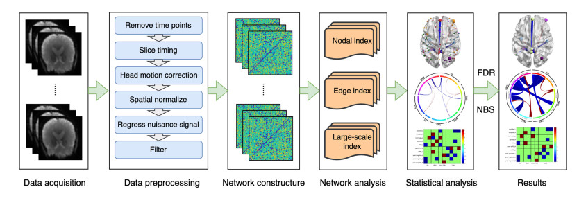
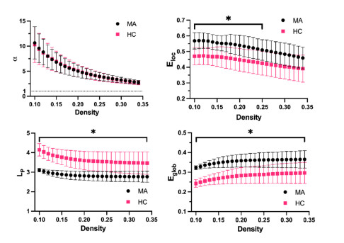
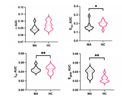
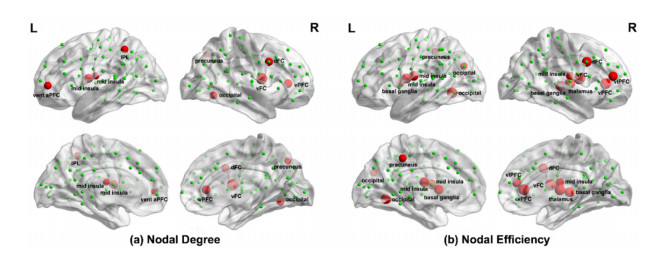
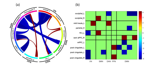
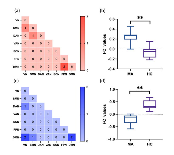
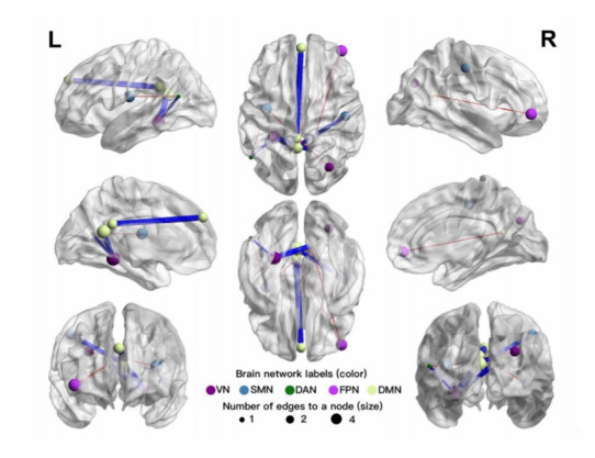
Our aim was to explore the aberrant intrinsic functional topology in methamphetamine-dependent individuals after six months of abstinence using resting-state functional magnetic imaging (rs-fMRI). Eleven methamphetamines (MA) abstainers who have abstained for six months and eleven healthy controls (HC) were recruited for rs-fMRI examination. The graph theory and functional connectivity (FC) analysis were employed to investigate the aberrant intrinsic functional brain topology between the two groups at multiple levels. Compared with the HC group, the characteristic shortest path length ($ {L}_{p} $) showed a significant decrease at the global level, while the global efficiency ($ {E}_{glob} $) and local efficiency ($ {E}_{loc} $) showed an increase considerably. After FDR correction, we found significant group differences in nodal degree and nodal efficiency at the regional level in the ventral attentional network (VAN), dorsal attentional network (DAN), somatosensory network (SMN), visual network (VN) and default mode network (DMN). In addition, the NBS method presented the aberrations in edge-based FC, including frontoparietal network (FPN), subcortical network (SCN), VAN, DAN, SMN, VN and DMN. Moreover, the FC of large-scale functional brain networks revealed a decrease within the VN and SCN and between the networks. These findings suggest that some functions, e.g., visual processing skills, object recognition and memory, may not fully recover after six months of withdrawal. This leads to the possibility of relapse behavior when confronted with MA-related cues, which may contribute to explaining the relapse mechanism. We also provide an imaging basis for revealing the neural mechanism of MA-dependency after six months of abstinence.
Citation: Xiang Li, Jinyu Cong, Kunmeng Liu, Pingping Wang, Min Sun, Benzheng Wei. Aberrant intrinsic functional brain topology in methamphetamine-dependent individuals after six-months of abstinence[J]. Mathematical Biosciences and Engineering, 2023, 20(11): 19565-19583. doi: 10.3934/mbe.2023867
Our aim was to explore the aberrant intrinsic functional topology in methamphetamine-dependent individuals after six months of abstinence using resting-state functional magnetic imaging (rs-fMRI). Eleven methamphetamines (MA) abstainers who have abstained for six months and eleven healthy controls (HC) were recruited for rs-fMRI examination. The graph theory and functional connectivity (FC) analysis were employed to investigate the aberrant intrinsic functional brain topology between the two groups at multiple levels. Compared with the HC group, the characteristic shortest path length ($ {L}_{p} $) showed a significant decrease at the global level, while the global efficiency ($ {E}_{glob} $) and local efficiency ($ {E}_{loc} $) showed an increase considerably. After FDR correction, we found significant group differences in nodal degree and nodal efficiency at the regional level in the ventral attentional network (VAN), dorsal attentional network (DAN), somatosensory network (SMN), visual network (VN) and default mode network (DMN). In addition, the NBS method presented the aberrations in edge-based FC, including frontoparietal network (FPN), subcortical network (SCN), VAN, DAN, SMN, VN and DMN. Moreover, the FC of large-scale functional brain networks revealed a decrease within the VN and SCN and between the networks. These findings suggest that some functions, e.g., visual processing skills, object recognition and memory, may not fully recover after six months of withdrawal. This leads to the possibility of relapse behavior when confronted with MA-related cues, which may contribute to explaining the relapse mechanism. We also provide an imaging basis for revealing the neural mechanism of MA-dependency after six months of abstinence.

| [1] |
B. Han, W. M. Compton, C. M. Jones, E. B. Einstein, N. D. Volkow, Methamphetamine use, methamphetamine use disorder, and associated overdose deaths among US adults, JAMA psychiatry, 78 (2021), 1329–1342. https://doi.org/10.1001/jamapsychiatry.2021.2588 doi: 10.1001/jamapsychiatry.2021.2588

|
| [2] |
M. Shukla, B. Vincent, Methamphetamine abuse disturbs the dopaminergic system to impair hippocampal-based learning and memory: An overview of animal and human investigations, Neurosci. Biobehav. Rev., 131 (2021), 541–559. https://doi.org/10.1016/j.neubiorev.2021.09.016 doi: 10.1016/j.neubiorev.2021.09.016
|
| [3] |
V. Manja, A. Nrusimha, Y. Gao, A. Sheikh, M. McGovern, P. A. Heidenreich, et al., Methamphetamine-associated heart failure: A systematic review of observational studies, Heart, 109 (2023), 168–177. https://doi.org/10.1136/heartjnl-2022-321610 doi: 10.1136/heartjnl-2022-321610
|
| [4] |
C. W. Li, S. W. W. Ku, P. Y. Huang, L. Y. Chen, H. T. Wei, C. Strong, et al., Factors associated with methamphetamine dependency among men who have sex with men engaging in chemsex: Findings from the COMeT study in Taiwan, Int. J. Drug Policy, 93 (2021), 103119. https://doi.org/10.1016/j.drugpo.2021.103119 doi: 10.1016/j.drugpo.2021.103119
|
| [5] |
S. P. Xu, K. Zhang, T. Y. Luo, Development of the risk of relapse assessment scale for methamphetamine abusers in China, Drug Alcohol Depend., 227 (2021), 108992. https://doi.org/10.1016/j.drugalcdep.2021.108992 doi: 10.1016/j.drugalcdep.2021.108992
|
| [6] |
H. Yuan, X. Yu, X. Li, S. Qin, G. Liang, T. Bai, et al., Research on resting spontaneous brain activity and functional connectivity of acupuncture at uterine acupoints, Digital Chin. Med., 5 (2022), 59–67. https://doi.org/10.1016/j.dcmed.2022.03.006 doi: 10.1016/j.dcmed.2022.03.006
|
| [7] | X. Li, B. Wei, T. Li, N. Zhang, MwoA auxiliary diagnosis via RSN-based 3D deep multiple instance learning with spatial attention mechanism, in 2020 11th International Conference on Awareness Science and Technology (iCAST), IEEE, (2020), 1–6. https://doi.org/10.1109/iCAST51195.2020.9319486 |
| [8] |
A. P. Daiwile, S. Jayanthi, J. L. Cadet, Sex differences in methamphetamine use disorder perused from pre-clinical and clinical studies: Potential therapeutic impacts, Neurosci. Biobehav. Rev., 137 (2022), 104674. https://doi.org/10.1016/j.neubiorev.2022.104674 doi: 10.1016/j.neubiorev.2022.104674
|
| [9] |
H. Mizoguchi, K. Yamada, Methamphetamine use causes cognitive impairment and altered decision-making, Neurochem. Int., 124 (2019), 106–113. https://doi.org/10.1016/j.neuint.2018.12.019 doi: 10.1016/j.neuint.2018.12.019
|
| [10] |
S. Sabrini, G. Y. Wang, J. C. Lin, J. K. Ian, L. E. Curley, Methamphetamine use and cognitive function: A systematic review of neuroimaging research, Drug Alcohol Depend., 194 (2019), 75–87. https://doi.org/10.1016/j.drugalcdep.2018.08.041 doi: 10.1016/j.drugalcdep.2018.08.041
|
| [11] |
S. J. Nieto, L. A. Ray, Applying the addictions neuroclinical assessment to derive neurofunctional domains in individuals who use methamphetamine, Behav. Brain Res., 427 (2022), 113876. https://doi.org/10.1016/j.bbr.2022.113876 doi: 10.1016/j.bbr.2022.113876
|
| [12] |
G. X. Liang, X. Li, H. Yuan, M. Sun, S. J. Qin, B. Z. Wei, Abnormal static and dynamic amplitude of low-frequency fluctuations in multiple brain regions of methamphetamine abstainers, Math. Biosci. Eng., 20 (2023), 13318–13333. https://doi.org/10.3934/mbe.2023593 doi: 10.3934/mbe.2023593
|
| [13] |
Z. X. Zhang, L. He, S. C. Huang, L. D. Fan, Y. N. Li, P. Li, et al., Alteration of brain structure with long-term abstinence of methamphetamine by voxel-based morphometry, Front. Psychiatry, 9 (2018), 722. https://doi.org/10.3389/fpsyt.2018.00722 doi: 10.3389/fpsyt.2018.00722
|
| [14] |
X. T. Li, H. Su, N. Zhong, T. Z. Chen, J. Du, K. Xiao, et al., Aberrant resting-state cerebellar-cerebral functional connectivity in methamphetamine-dependent individuals after six months abstinence, Front. Psychiatry, 11 (2020), 191. https://doi.org/10.3389/fpsyt.2020.00191 doi: 10.3389/fpsyt.2020.00191
|
| [15] |
L. Fan, Q. Zhang, S. Liang, H. Li, Z. He, J. Sun, et al., Imaging changes in brain microstructural in long-term abstinent from methamphetamine-dependence (in Chinese), J. Cent. South Univ. (Med. Sci.), 44 (2019), 491–500. https://doi.org/10.11817/j.issn.1672-7347.2019.05.004 doi: 10.11817/j.issn.1672-7347.2019.05.004
|
| [16] |
X. Y. Qi, Y. Y. Wang, Y. Z. Lu, Q. Zhao, Y. F. Chen, C. L. Zhou, et al., Enhanced brain network flexibility by physical exercise in female methamphetamine users, Cognit. Neurodyn., 2022 (2022), 1–17. https://doi.org/10.1007/s11571-022-09848-5 doi: 10.1007/s11571-022-09848-5
|
| [17] |
C. Y. Jia, Q. F. Long, T. Ernst, Y. Q. Shang, L. D. Chang, T. Adali, Independent component and graph theory analyses reveal normalized brain networks on resting-state functional MRI after working memory training in people with HIV, J. Magn. Reson. Imaging, 57 (2023), 1552–1564. https://doi.org/10.1002/jmri.28439 doi: 10.1002/jmri.28439
|
| [18] |
O. Sporns, Graph theory methods: applications in brain networks, Dialogues Clin. Neurosci., 20 (2018), 111–121. https://doi.org/10.31887/DCNS.2018.20.2/osporns doi: 10.31887/DCNS.2018.20.2/osporns
|
| [19] |
W. Li, L. Wang, Z. Lyu, J. J. Chen, Y. B. Li, Y. C. Sun, et al., Difference in topological organization of white matter structural connectome between methamphetamine and heroin use disorder, Behav. Brain Res., 422 (2022), 113752. https://doi.org/10.1016/j.bbr.2022.113752 doi: 10.1016/j.bbr.2022.113752
|
| [20] |
M. Siyah Mansoory, M. A. Oghabian, A. H. Jafari, A. Shahbabaie, Analysis of resting-state fMRI topological graph theory properties in methamphetamine drug users applying box-counting fractal dimension, Basic Clin. Neurosci., 8 (2017), 371–385. https://doi.org/10.18869/nirp.bcn.8.5.371 doi: 10.18869/nirp.bcn.8.5.371
|
| [21] |
Y. A. Zhou, Y. Hu, Q. J. Wang, Z. Yang, J. G. Li, Y. J. Ma, et al., Association between white matter microstructure and cognitive function in patients with methamphetamine use disorder, Hum. Brain Mapp., 44 (2023), 304–314. https://doi.org/10.1002/hbm.26020 doi: 10.1002/hbm.26020
|
| [22] |
M. S. Mansoory, A. Allahverdy, M. Behboudi, M. Khodamoradi, Local efficiency analysis of restingstate functional brain network in methamphetamine users, Behav. Brain Res., 434 (2022), 114022. https://doi.org/10.1016/j.bbr.2022.114022 doi: 10.1016/j.bbr.2022.114022
|
| [23] |
F. Miraglia, F. Vecchio, C. Pappalettera, L. Nucci, M. Cotelli, E. Judica, et al., Brain connectivity and graph theory analysis in Alzheimer's and Parkinson's Disease: The contribution of electrophysiological techniques, Brain Sci., 12 (2022), 402. https://doi.org/10.3390/brainsci12030402 doi: 10.3390/brainsci12030402
|
| [24] |
C. G. Yan, X. D. Wang, X. N. Zuo, Y. F. Zang, DPABI: Data processing & analysis for (resting-state) brain imaging, Neuroinformatics, 14 (2016), 339–351. https://doi.org/10.1007/s12021-016-9299-4 doi: 10.1007/s12021-016-9299-4
|
| [25] |
C. G. Yan, R. C. Craddock, Y. He, M. P. Milham, Addressing head motion dependencies for small-world topologies in functional connectomics, Front. Hum. Neurosci., 7 (2013), 910. https://doi.org/10.3389/fnhum.2013.00910 doi: 10.3389/fnhum.2013.00910
|
| [26] |
C. Yan, Y. Zang, DPARSF: A MATLAB toolbox for "pipeline" data analysis of resting-state fMRI, Front. Syst. Neurosci., 4 (2010), 13. https://doi.org/10.3389/fnsys.2010.00013 doi: 10.3389/fnsys.2010.00013
|
| [27] |
N. U. F. Dosenbach, B. Nardos, A. L. Cohen, D. A. Fair, J. D. Power, J. A. Church, et al., Prediction of individual brain maturity using fMRI, Science, 329 (2010), 1358–1361. https://doi.org/10.1126/science.1194144 doi: 10.1126/science.1194144
|
| [28] |
M. Koutrouli, E. Karatzas, D. Paez-Espino, G. A. Pavlopoulos, A Guide to conquer the biological network Era using graph theory, Front. Bioeng. Biotechnol., 8 (2020), 34. https://doi.org/10.3389/fbioe.2020.00034 doi: 10.3389/fbioe.2020.00034
|
| [29] |
B. T. T. Yeo, F. M. Krienen, J. Sepulcre, M. R. Sabuncu, D. Lashkari, M. Hollinshead, et al., The organization of the human cerebral cortex estimated by intrinsic functional connectivity, J. Neurophysiol., 106 (2011), 1125–1165. https://doi.org/10.1152/jn.00338.2011 doi: 10.1152/jn.00338.2011
|
| [30] |
G. Li, Y. D. Luo, Z. R. Zhang, Y. T. Xu, W. D. Jiao, Y. H. Jiang, et al., Effects of mental fatigue on < i > Small-World < /i > brain functional network organization, Neural Plast., 2019 (2019), 1716074. https://doi.org/10.1155/2019/1716074 doi: 10.1155/2019/1716074
|
| [31] |
L. J. Nestor, D. G. Ghahremani, E. D. London, Reduced neural functional connectivity during working memory performance in methamphetamine use disorder, Drug Alcohol Depend., 243 (2023), 109764. https://doi.org/10.1016/j.drugalcdep.2023.109764 doi: 10.1016/j.drugalcdep.2023.109764
|
| [32] |
M. Ahmadlou, K. Ahmadi, M. Rezazade, E. Azad-Marzabadi, Global organization of functional brain connectivity in methamphetamine abusers, Clin. Neurophysiol., 124 (2013), 1122–1131. https://doi.org/10.1016/j.clinph.2012.12.003 doi: 10.1016/j.clinph.2012.12.003
|
| [33] |
S. Arvin, A. N. Glud, K. Yonehara, Short- and long-range connections differentially modulate the dynamics and state of small-world networks, Front. Comput. Neurosci., 15 (2022), 783474. https://doi.org/10.3389/fncom.2021.783474 doi: 10.3389/fncom.2021.783474
|
| [34] |
Y. Liu, Q. Li, T. Y. Zhang, L. Wang, Y. R. Wang, J. J. Chen, et al., Differences in small-world networks between methamphetamine and heroin use disorder patients and their relationship with psychiatric symptoms, Brain Imaging Behav., 16 (2022), 1973–1982. https://doi.org/10.1007/s11682-022-00667-0 doi: 10.1007/s11682-022-00667-0
|
| [35] |
H. Khajehpour, B. Makkiabadi, H. Ekhtiari, S. Bakht, A. Noroozi, F. Mohagheghian, Disrupted resting-state brain functional network in methamphetamine abusers: A brain source space study by EEG, PLoS One, 14 (2019), e0226249. https://doi.org/10.1371/journal.pone.0226249 doi: 10.1371/journal.pone.0226249
|
| [36] |
F. X. Vollenweider, K. H. Preller, Psychedelic drugs: neurobiology and potential for treatment of psychiatric disorders, Nat. Rev. Neurosci., 21 (2020), 611–624. https://doi.org/10.1038/s41583-020-0367-2 doi: 10.1038/s41583-020-0367-2
|
| [37] |
B. Kim, J. Yun, B. Park, Methamphetamine-induced neuronal damage: Neurotoxicity and neuroinflammation, Biomol. Ther., 28 (2020), 381–388. https://doi.org/10.4062/biomolther.2020.044 doi: 10.4062/biomolther.2020.044
|
| [38] |
J. Zhang, H. Su, J. Y. Tao, Y. Xie, Y. M. Sun, L. R. Li, et al., Relationship of impulsivity and depression during early methamphetamine withdrawal in Han Chinese population, Addict. Behav., 43 (2015), 7–10. https://doi.org/10.1016/j.addbeh.2014.10.032 doi: 10.1016/j.addbeh.2014.10.032
|
| [39] |
A. Scalabrini, B. Vai, S. Poletti, S. Damiani, C. Mucci, C. Colombo, et al., All roads lead to the default-mode network-global source of DMN abnormalities in major depressive disorder, Neuropsychopharmacology, 45 (2020), 2058–2069. https://doi.org/10.1038/s41386-020-0785-x doi: 10.1038/s41386-020-0785-x
|
| [40] |
B. L. Foster, S. R. Koslov, L. Aponik-Gremillion, M. E. Monko, B. Y. Hayden, S. R. Heilbronner, A tripartite view of the posterior cingulate cortex, Nat. Rev. Neurosci., 24 (2023), 173–189. https://doi.org/10.1038/s41583-022-00661-x doi: 10.1038/s41583-022-00661-x
|
| [41] |
C. Caldinelli, R. Cusack, The fronto-parietal network is not a flexible hub during naturalistic cognition, Hum. Brain Mapp., 43 (2022), 750–759. https://doi.org/10.1002/hbm.25684 doi: 10.1002/hbm.25684
|
| [42] |
H. Zheng, Q. Zhou, J. J. Yang, Q. Lu, H. D. Qiu, C. He, et al., Altered functional connectivity of the default mode and frontal control networks in patients with insomnia, CNS Neurosci. Ther., 29 (2023), 2318–2326. https://doi.org/10.1111/cns.14183 doi: 10.1111/cns.14183
|
| [43] |
R. De Micco, N. Piramide, F. Di Nardo, M. Siciliano, M. Cirillo, A. Russo, et al., Resting-state network connectivity changes in drug-naive Parkinson's disease patients with probable REM sleep behavior disorder, J. Neural Transm., 130 (2023), 43–51. https://doi.org/10.1007/s00702-022-02565-7 doi: 10.1007/s00702-022-02565-7
|
| [44] |
S. Tikoo, F. Cardona, S. Tommasin, C. Giannì, G. Conte, N. Upadhyay, et al., Resting-state functional connectivity in drug-naive pediatric patients with Tourette syndrome and obsessive-compulsive disorder, J. Psychiatr. Res., 129 (2020), 129–140. https://doi.org/10.1016/j.jpsychires.2020.06.021 doi: 10.1016/j.jpsychires.2020.06.021
|
| [45] |
G. Dong, E. DeVito, J. Huang, X. Du, Diffusion tensor imaging reveals thalamus and posterior cingulate cortex abnormalities in internet gaming addicts. J. Psychiatr. Res., 46 (2012), 1212–1216. https://doi.org/10.1016/j.jpsychires.2012.05.015 doi: 10.1016/j.jpsychires.2012.05.015
|
| [46] |
Y. Katsumi, D. Putcha, R. Eckbo, B. Wong, M. Quimby, S. McGinnis, et al., Anterior dorsal attention network tau drives visual attention deficits in posterior cortical atrophy, Brain, 146 (2023), 295–306. https://doi.org/10.1093/brain/awac245 doi: 10.1093/brain/awac245
|
| [47] |
H. Y. Tan, T. Z. Chen, J. Du, R. J. Li, H. F. Jiang, C. L. Deng, et al., Drug-related virtual reality cue reactivity is associated with gamma activity in reward and executive control circuit in methamphetamine use disorders, Arch. Med. Res., 50 (2019), 509–517. https://doi.org/10.1016/j.arcmed.2019.09.003 doi: 10.1016/j.arcmed.2019.09.003
|
| [48] |
H. C. Zhao, M. J. Ge, O. Turel, A. Bechara, Q. H. He, Brain modular connectivity interactions can predict proactive inhibition in smokers when facing smoking cues, Addict. Biol., 28 (2023), e13284. https://doi.org/10.1111/adb.13284 doi: 10.1111/adb.13284
|
| [49] |
S. Yilmaz, Impaired biological rhythm in men with methamphetamine use disorder: The relationship with sleep quality and depression, J. Subst. Use, 28 (2023), 280–286. https://doi.org/10.1080/14659891.2022.2098847 doi: 10.1080/14659891.2022.2098847
|
| [50] |
L. Cerliani, M. Mennes, R. M. Thomas, A. Di Martino, M. Thioux, C. Keysers, Increased functional connectivity between subcortical and cortical resting-state networks in autism spectrum disorder, JAMA Psychiatry, 72 (2015), 767–777. https://doi.org/10.1001/jamapsychiatry.2015.0101 doi: 10.1001/jamapsychiatry.2015.0101
|
| [51] |
A. Moaveni, Y. F. Feyzi, S. T. Rahideh, R. Arezoomandan, The relationship between serum brain-derived neurotrophic level and neurocognitive functions in chronic methamphetamine users, Neurosci. Lett., 772 (2022), 136478. https://doi.org/10.1016/j.neulet.2022.136478 doi: 10.1016/j.neulet.2022.136478
|
| [52] |
R. Nusslock, G. H. Brody, C. C. Armstrong, A. L. Carroll, L. H. Sweet, T. Y. Yu, et al., Higher peripheral inflammatory signaling associated with lower resting-state functional brain connectivity in emotion regulation and central executive networks, Biol. Psychiatry, 86 (2019), 153–162. https://doi.org/10.1016/j.biopsych.2019.03.968 doi: 10.1016/j.biopsych.2019.03.968
|
| [53] |
M. Esposito, M. Tamietto, G. C. Geminiani, A. Celeghin, A subcortical network for implicit visuo-spatial attention: Implications for Parkinson's disease, Cortex, 141 (2021), 421–435. https://doi.org/10.1016/j.cortex.2021.05.003 doi: 10.1016/j.cortex.2021.05.003
|
| [54] |
Y. Z. Sun, Y. Ding, T. Y. Yu, C. Y. Chen, P. Li, X. G. Yang, et al., Effect of Tiaoshen acupuncture on anxiety after methamphetamine withdrawal (in Chinese), Chin. Acupunct. Moxibust., 42 (2022), 277–280. https://doi.org/10.13703/j.0255-2930.20210213-k0001 doi: 10.13703/j.0255-2930.20210213-k0001
|
| [55] |
R. K. Meleppat, C. R. Fortenbach, Y. F. Jian, E. S. Martinez, K. Wagner, B. S. Modjtahedi, et al., In vivo imaging of retinal and choroidal morphology and vascular plexuses of vertebrates using swept-source optical coherence tomography, Transl. Vision Sci. Technol., 11 (2022), 11. https://doi.org/10.1167/tvst.11.8.11 doi: 10.1167/tvst.11.8.11
|
| [56] |
R. K. Meleppat, K. E. Ronning, S. J. Karlen, M. E. Burns, E. N. Pugh, R. J. Zawadzki, In vivo multimodal retinal imaging of disease-related pigmentary changes in retinal pigment epithelium, Sci. Rep., 11 (2021), 16252. https://doi.org/10.1038/s41598-021-95320-z doi: 10.1038/s41598-021-95320-z
|
| [57] |
R. K. Meleppat, P. F. Zhang, M. J. Ju, S. K. Manna, Y. Jian, E. N. Pugh, et al., Directional optical coherence tomography reveals melanin concentration-dependent scattering properties of retinal pigment epithelium, J. Biomed. Opt., 24 (2019), 066011. https://doi.org/10.1117/1.Jbo.24.6.066011 doi: 10.1117/1.Jbo.24.6.066011
|
| [58] |
K. M. Ratheesh, L. K. Seah, V. M. Murukeshan, Spectral phase-based automatic calibration scheme for swept source-based optical coherence tomography systems, Phys. Med. Biol., 61 (2016), 7652–7663. https://doi.org/10.1088/0031-9155/61/21/7652 doi: 10.1088/0031-9155/61/21/7652
|

Figures(8) / Tables(4)

Xiang Li, Jinyu Cong, Kunmeng Liu, Pingping Wang, Min Sun, Benzheng Wei. Aberrant intrinsic functional brain topology in methamphetamine-dependent individuals after six-months of abstinence[J]. Mathematical Biosciences and Engineering, 2023, 20(11): 19565-19583. doi: 10.3934/mbe.2023867


 DownLoad: